Page 716 - The Mechatronics Handbook

0066_Frame_C23 Page 24 Wednesday, January 9, 2002 1:53 PM

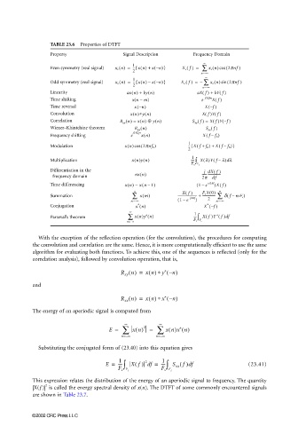
TABLE 23.6 Properties of DTFT
Property Signal Description Frequency Domain
∞
1
(
Even symmetry (real signal) x e n() = -- xn() +{ x – n)} X e f() = ∑ x e n() cos ( 2πnf )
2
n=∞
–
∞
1
(
Odd symmetry (real signal) x o n() = -- xn() –{ x – n)} X o f() = – ∑ x o n() sin ( 2πnf )
2
n=∞
–
Linearity ax n() + by n() aX f() + bY f()
Time shifting x(n − m) e −j2πfm X f()
(
(
Time reversal x – n) X – )
f
Convolution x n() ∗y n() X f() Y f()
(
Correlation R xy n() = x n() ⊕ y n() S xy f() = X f() Y f )
–
Wiener–Khintchine theorem R xx n() S xx f()
j2πf 0 n
(
Frequency shifting e xn() X f – )
f 0
(
Modulation xn() cos ( 2pnf 0 ) 1 -- Xf +({ f 0 ) + Xf – )}
f 0
2
1
Multiplication x n() n() ---- ∫ X λ()Yf λ–( ) λ
d
y
F s F s
Differentiation in the j dX f()
frequency domain nx n() ----------------------
2π
df
Time differencing x n() − x n –( 1) ( 1 – e – j2pf )Xf()
∞
Xf()
n
(
----------------
Summation ∑ xm() ------------------------ + F s X 0() ∑ δ f – mF s )
–
j2πf
m=∞ ( 1 – e ) 2 m=∞
–
–
∗
∗
(
Conjugation x n() X – )
f
∞ 1
∗
∗
d
f
Parseval’s theorem ∑ xn()y n() ---- ∫ Xf()Y () f
n=∞ F s F s
–
With the exception of the reflection operation (for the convolution), the procedures for computing
the convolution and correlation are the same. Hence, it is more computationally efficient to use the same
algorithm for evaluating both functions. To achieve this, one of the sequences is reflected (only for the
correlation analysis), followed by convolution operation, that is,
R xy n() = xn() ∗ y – n)
(
∗
and
R xx n() = xn() ∗ x – n)
(
∗
The energy of an aperiodic signal is computed from
∞ ∞
E = ∑ x n() 2 = ∑ xn()x n()
∗
n=∞ n=∞
–
–
Substituting the conjugated form of (23.40) into this equation gives
1
1
E = ---- ∫ Xf() d = ---- ∫ S xx f() f (23.41)
2
f
d
F s F F s F
s s
This expression relates the distribution of the energy of an aperiodic signal to frequency. The quantity
2
|X(f )| is called the energy spectral density of x(n). The DTFT of some commonly encountered signals
are shown in Table 23.7.
©2002 CRC Press LLC