Page 718 - The Mechatronics Handbook

0066_Frame_C23 Page 26 Wednesday, January 9, 2002 1:53 PM

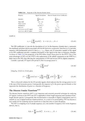
TABLE 23.8 Properties of the Discrete Fourier Series
Property Signal Description Discrete Fourier Series Coefficients
Q Q
Linearity ∑ β m x m n() ∑ β m c m,k
m=0 m=0
(
Time shift xn – m) c k W N km
(
Time-reversal x – n) c −k
– mn
Modulation xn()W N c k−m
Real x(n) xn() c k = c k ∗
()
x e (n) is an even DT signal x e n() Re c k
{
()}
x 0 (n) is an odd DT signal x o n() j Im c k
results in
N−1
1
c k = ---- ∑ xn()W N , k = 0, 1, 2,…, N 1 (23.43)
kn
–
N
n=0
The DFS coefficients {c k } provide the description of x(n) in the frequency domain since c k represents
the amplitude and phase spectra associated with the kth harmonic component. Note that {c k } is a periodic
sequence with fundamental period N, that is, c k = c k+N . Hence, any N consecutive samples of the signal
or its DFS coefficients provide a complete description of the signal in the time or frequency domains.
As shown in Table 23.8, the properties of the DFS follow closely those given for the DTFT. One of the
main advantages of DFS over the DTFT is the replacement of the infinite summation in the DTFT by a
finite sum in the DFS, thus allowing the computations of DFS and inverse DFS by digital computers.
Consider a periodic DT signal with period N, then its average power is

N−1
1
P = ---- ∑ xn() 2 (23.44)
N
n=0
Using Eq. (23.42) in (23.44) gives


1
∑
∑
∑
1
∑
∗
kn
P = ---- N−1 xn()x n() = ---- N−1 xn()  N−1 c k W N  = N−1 c k 2 (23.45)
∗
N N  
n=0 n=0 k=0 k=0
This is a Parseval’s relation for the DT periodic signals, which indicates that the average power in x(n)
2
is the sum of the harmonics power. Consequently, the sequence |c k | is the power spectral density as this
represents the distribution of power as a function of frequency.
The Discrete Fourier Transform 6,8,13
The discrete Fourier transform (DFT) is an important and extremely powerful technique for analyzing
DT signals. Contrary to the DTFT, the DFT is applicable to finite-length sequences and it produces finite-
length discrete spectra. Consequently, this transformation is amenable to digital computations and it is
suitable for use in digital hardware implementations. As a result of its practicability, DFT has become a
very useful tool for analyzing various waveforms or data that arise in many disciplines.
The DFT is a mapping of an N sample sequence, x(n), into another N sequence X(k) in the frequency
domain, that is,
N−1
kn
Xk() = ∑ xn()W N , k = 0, 1,…,N 1 (23.46)
–
n=0
©2002 CRC Press LLC