Page 723 - The Mechatronics Handbook

0066_Frame_C23 Page 31 Wednesday, January 9, 2002 1:53 PM

TABLE 23.10 Properties of the z Transform
z transform ({f k }) = F(z)
Convolution ({f k ∗ g k }) = ({f k }) ⋅ ({g k })
({f k ⋅ g k }) = ({f k }) ∗ ({g k })
Forward shift ({f k+1 }) = z ({f k }) = zF(z)
−1
Backward shift ({f k−1 }) = ({f k }) = z F(z)
Linearity ({af k + bg k }) = a ({f k }) + b ({g k })
k
−1
Multiplication ({a f k }) = F(a z)
1
–
Final value lim f k = lim ( 1 – z )Fz()
k→∞ k→1
Initial value f 0 = lim Fz()
z→∞
Time Domain z Transform
 1, k = 0
Impulse d k =  {δ k } = 1, z ∈ C
 0, k ≠ 0
 0, k < 0 z
(
Step function s k =  s k ) = -----------, z > 1
 1, k ≥ 0 z – 1
z
Ramp function x k = k ⋅ σ k Xz() = ------------------, z > 1
( z – 1) 2
z
k
Exponential x k = a ⋅ σ k Xz() = -----------, z > a
z – a
z sin
w
Sinusoid x k = sin ωk ⋅ σ k Xz() = --------------------------------------, z > 1
2
z – 2z cos w + 1
x(t) {x }
Sampling k
device

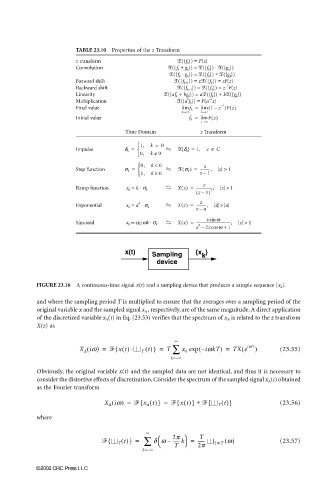
FIGURE 23.16 A continuous-time signal x(t) and a sampling device that produces a sample sequence {x k }.

and where the sampling period T is multiplied to ensure that the averages over a sampling period of the
original variable x and the sampled signal x ∆ , respectively, are of the same magnitude. A direct application
of the discretized variable x ∆ (t) in Eq. (23.53) verifies that the spectrum of x ∆ is related to the z transform
X(z) as

∞
⋅
{
(
(
(
X ∆ iw) = xt() T t()} = T ∑ x k exp – iwkT) = TX e iwT ) (23.55)
k=−∞
Obviously, the original variable x(t) and the sampled data are not identical, and thus it is necessary to
consider the distortive effects of discretization. Consider the spectrum of the sampled signal x ∆ (t) obtained
as the Fourier transform
{
{
X ∆ iw) = x ∆ t()} = xt()} ∗ { T t()} (23.56)
(
where
∞
T

------ k =
{ T t()} = ∑ dw – 2p  ------ 2p/T w() (23.57)
T 

k=−∞ 2p
©2002 CRC Press LLC