Page 728 - The Mechatronics Handbook

0066_Frame_C23 Page 36 Wednesday, January 9, 2002 1:55 PM

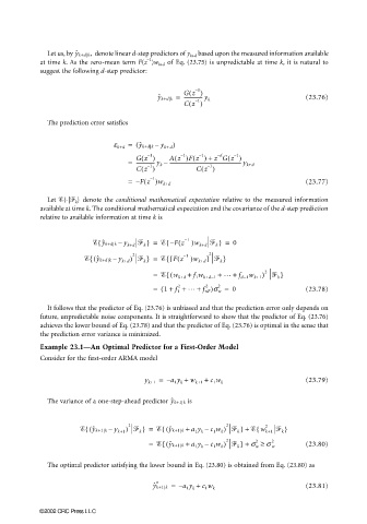
Let us, by y ˆ k+d|k, denote linear d-step predictors of y k+d based upon the measured information available
−1
at time k. As the zero-mean term F(z )w k+d of Eq. (23.75) is unpredictable at time k, it is natural to
suggest the following d-step predictor:

(
1
–
y ˆ k+d|k = Gz ) (23.76)
--------------- y k
Cz ( – 1 )
The prediction error satisfies
e k+d = ( y ˆ k+d|k – y k+ d )

(
(
Gz ( – 1 ) Az )Fz ) + z Gz )
(
–
d
–
–
1
–
1
1
= --------------- y k – ----------------------------------------------------------- y k+d
(
Cz ) Cz )
(
1
1
–
–
(
= – Fz )w k+d (23.77)
–
1
Let {⋅| k } denote the conditional mathematical expectation relative to the measured information
available at time k. The conditional mathematical expectation and the covariance of the d-step prediction
relative to available information at time k is
(
{
{
–
1
y ˆ k+dk – y k+d k } = – Fz )w k+d k } = 0
2
(
{
(
2
{
–
1
y ˆ k+dk – y k+d ) k } = [ Fz )w k+d ] k }
= ( w k+d + f 1 w k+d−1 + … + f d−1 w k+1 ) k }
{
2
2
2
2
= ( 1 + f 1 + … + f nF )s w = 0 (23.78)
It follows that the predictor of Eq. (23.76) is unbiased and that the prediction error only depends on
future, unpredictable noise components. It is straightforward to show that the predictor of Eq. (23.76)
achieves the lower bound of Eq. (23.78) and that the predictor of Eq. (23.76) is optimal in the sense that
the prediction error variance is minimized.
Example 23.1—An Optimal Predictor for a First-Order Model
Consider for the first-order ARMA model
y k+1 = – a 1 y k + w k+1 + c 1 w k (23.79)
The variance of a one-step-ahead predictor y ˆ k+1 k is
2
{
{
2
{
(
2
y ˆ k+1 k – y k+1 ) k } = ( y ˆ k+1 k + a 1 y k – c 1 w k ) k } + w k+1 k }
2
2
= ({ y ˆ k+1 k + a 1 y k – c 1 w k ) k } + σ w ≥ σ w 2 (23.80)
The optimal predictor satisfying the lower bound in Eq. (23.80) is obtained from Eq. (23.80) as
o
y ˆ k+1 k = – a 1 y k + c 1 w k (23.81)
©2002 CRC Press LLC