Page 730 - The Mechatronics Handbook

0066_Frame_C23 Page 38 Wednesday, January 9, 2002 1:55 PM

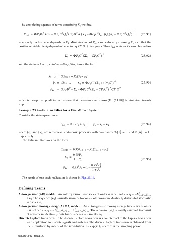
By completing squares of terms containing K k we find

1 T
T
T
–
P k+1 = ΦP k Φ + Σ v – ΦP k C Q k CP k Φ + ( K k – ΦP k C Q k )Q k K k – ΦP k C Q k ) (23.91)
(
–
1
–
1
T
T
T
where only the last term depends on K k . Minimization of P k+1 can be done by choosing K k such that the
positive semidefinite K k -dependent term in Eq. (23.91) disappears. Thus P k+1 achieves its lower bound for
(
K k = ΦP k C Σ w + CP k C ) 1 (23.92)
T –
T
and the Kalman filter (or Kalman–Bucy filter) takes the form
x ˆ k+1 k = Φx ˆ kk−1 – K k y ˆ k – y k )
(
y ˆ k = Cx ˆ kk−1, K k = ΦP k C Σ w + CP k C ) 1 (23.93)
(
T –
T
T –
1
(
T
P k+1 = ΦP k Φ + Σ v – ΦP k C Σ w + CP k C ) CP k Φ T
T
which is the optimal predictor in the sense that the mean square error (Eq. (23.88)) is minimized in each
step.
Example 23.2—Kalman Filter for a First-Order System
Consider the state-space model
x k+1 = 0.95x k + v k , y k = x k + w k (23.94)
where {v k } and {w k } are zero-mean white-noise processes with covariances {v k = 1 and {w k } = 1,
2
2
respectively.
The Kalman filter takes on the form
(
x ˆ k+1|k = 0.95x ˆ k|k−1 – K k x ˆ k|k−1 – y k )
K k = 0.95P k
---------------
1 + P k (23.95)
2 2
P k+1 = 0.95 P k + 1 – 0.95 P k
2
-----------------
1 + P k
The result of one such realization is shown in Fig. 23.19.

Defining Terms
n
–
Autoregressive (AR) model: An autoregressive time series of order n is defined via y k = Σ m=1 a m y k−m
+ w k . The sequence {w k } is usually assumed to consist of zero-mean identically distributed stochastic
variables w k .
Autoregressive moving average (ARMA) model: An autoregressive moving average time series of order
n n
– c m w k−m . The sequence {w k } is usually assumed to consist
n is defined via y k = Σ m=1 a m y k−m + Σ m=0
of zero-mean identically distributed stochastic variables w k .
Discrete Laplace transform: The discrete Laplace transform is a counterpart to the Laplace transform
with application to discrete signals and systems. The discrete Laplace transform is obtained from
the z transform by means of the substitution z = exp(sT), where T is the sampling period.

©2002 CRC Press LLC