Page 725 - The Mechatronics Handbook

0066_Frame_C23 Page 33 Wednesday, January 9, 2002 1:55 PM

The Discrete Fourier Transform
Consider a finite length sequence {x k } N−1 that is zero outside the interval 0 ≤ k ≤ N − 1. Evaluation of
k=0
the z transform X(z) at N equally spaced points on the unit circle z = exp(iω k T) = exp[i(2π/NT)kT] for
k = 0, 1,…, N − 1 defines the discrete Fourier transform (DFT) of a signal x with a sampling period h and
N measurements:
N−1
{
(
X k = DFT xkT)} = ∑ x l exp – ( iw k lT) = Xe iw T ) (23.60)
(
k
l=0
N−1
Notice that the discrete Fourier transform {X k } k=0 is only defined at the discrete frequency points
2p
w k = -------- k, for k = 0, 1,…, N 1 (23.61)
–
NT
In fact, the discrete Fourier transform adapts the Fourier transform and the z transform to the practical
requirements of finite measurements. Similar properties hold for the discrete Laplace transform with z =
exp(sT), where s is the Laplace transform variable.
The Transfer Function

Consider the following discrete-time linear system with input sequence {u k } (stimulus) and output sequence
{y k } (response). The dependency of the output of a linear system is characterized by the convolution-
type equation and its z transform,
∞ k
y k ∑ h m u k−m + v k = ∑ h k−m u m + v k , k = …, −1, 0, 1, 2,…
=
m=0 m=−∞ (23.62)
Yz() = Hz()Uz() + Vz()

where the sequence {v k } represents some external input of errors and disturbances and with Y(z) = {y},
∞
U(z) = {u}, V(z) = {v} as output and inputs. The weighting function h(kT) = {h k } k=0 , which is zero
for negative k and for reasons of causality is sometimes called pulse response of the digital system (compare
impulse response of continuous-time systems). The pulse response and its z transform, the pulse transfer
function,
∞
(
{
Hz() = hkT)} = ∑ h k z k – (23.63)
k=0
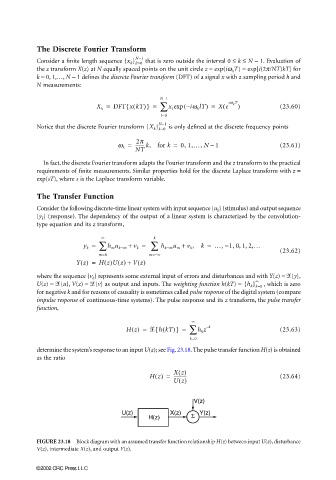
determine the system’s response to an input U(z); see Fig. 23.18. The pulse transfer function H(z) is obtained
as the ratio
Xz()
Hz() = ----------- (23.64)
Uz()

V(z)
U(z) X(z) Σ Y(z)
H(z)

FIGURE 23.18 Block diagram with an assumed transfer function relationship H(z) between input U(z), disturbance
V(z), intermediate X(z), and output Y(z).

©2002 CRC Press LLC