Page 838 - The Mechatronics Handbook

066_Frame_C26 Page 23 Wednesday, January 9, 2002 1:59 PM

Root Loci with Pade Approximations of Orders 1, 2, and 3
25
l = 1
K = 20.6
20
l = 3
15

l = 2
10
K = 16.1
5
0
−5
−10
−15
−20
−25
−12 −10 −8 −6 −4 −2 0 2
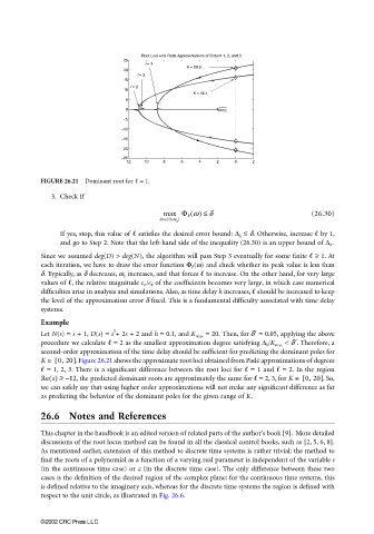
FIGURE 26.21 Dominant root for = 1.

3. Check If

max Φ w() ≤ d (26.30)
w [ 0,w ]
∈
x
If yes, stop, this value of satisfies the desired error bound: ∆ h ≤ d. Otherwise, increase by 1,
and go to Step 2. Note that the left-hand side of the inequality (26.30) is an upper bound of ∆ h .
Since we assumed deg(D) > deg(N), the algorithm will pass Step 3 eventually for some finite ≥ 1. At
each iteration, we have to draw the error function Φ (w) and check whether its peak value is less than
d. Typically, as d decreases, w x increases, and that forces to increase. On the other hand, for very large
values of , the relative magnitude c 0 /c of the coefficients becomes very large, in which case numerical
difficulties arise in analysis and simulations. Also, as time delay h increases, should be increased to keep
the level of the approximation error d fixed. This is a fundamental difficulty associated with time delay
systems.
Example
2
Let N(s) = s + 1, D(s) = s + 2s + 2 and h = 0.1, and K max = 20. Then, for = 0.05, applying the above′
d
procedure we calculate = 2 as the smallest approximation degree satisfying ∆ h /K max < . Therefore, ad′
second-order approximation of the time delay should be sufficient for predicting the dominant poles for
K ∈ [ 0, 20] . Figure 26.21 shows the approximate root loci obtained from Padé approximations of degrees
= 1, 2, 3. There is a significant difference between the root loci for = 1 and = 2. In the region
Re s() ≥ – 12 , the predicted dominant roots are approximately the same for = 2, 3, for K ∈ [ 0, 20] . So,
we can safely say that using higher order approximations will not make any significant difference as far
as predicting the behavior of the dominant poles for the given range of K.

26.6 Notes and References

This chapter in the handbook is an edited version of related parts of the author’s book [9]. More detailed
discussions of the root locus method can be found in all the classical control books, such as [2, 5, 6, 8].
As mentioned earlier, extension of this method to discrete time systems is rather trivial: the method to
find the roots of a polynomial as a function of a varying real parameter is independent of the variable s
(in the continuous time case) or z (in the discrete time case). The only difference between these two
cases is the definition of the desired region of the complex plane: for the continuous time systems, this
is defined relative to the imaginary axis, whereas for the discrete time systems the region is defined with
respect to the unit circle, as illustrated in Fig. 26.6.

©2002 CRC Press LLC