Page 841 - The Mechatronics Handbook

0066_frame_C27 Page 2 Wednesday, January 9, 2002 7:10 PM

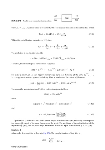
FIGURE 27.1 A stable linear constant coefficient system.

where p i , i = 1, 2,…,n, are assumed to be distinct poles. The Laplace transform of the output Y(s) is then

U 0
Ys() = Gs()Us() = Gs()------------- (27.4)
–
sjw
Taking the partial fraction expansion of Y(s) gives

a
Ys() = ------------- + … + ------------- + ------------- (27.5)
k 1
k n
s + p 1 s + p n sjw
–
The coefficient α can be determined by
a = ( [ sjw)Ys()] = [ U 0 Gs()] = U 0 Gjw)
(
–
s=jw s=jw
Therefore, the inverse Laplace transform of Y(s) yields

(
yt() = k 1 e −p t + … + k n e – p t + U 0 Gjw)e jwt , t ≥ 0 (27.6)
1
n
– p t i
For a stable system, all −p i have negative nonzero real parts and, therefore, all the terms k i e , i = 1,
2,…,n, approach zero as t approaches infinity. Thus, at steady state, the output y(t) becomes
(
(
y ss t() = lim yt() = U 0 Gjw)e jwt = U 0 Gjw) e j wt+f) (27.7)
(
t → ∞
The sinusoidal transfer function, G(jω), is written in exponential form
(
(
Gjw) = Gjw) e j f
where

(
(
[
[
Gjw) = { Re Gjw)]} + { Im Gjw)]} 2 (27.8a)
(
2
and
1Im Gjw([ )]
f = ∠ Gjw) = tan ---------------------------- (27.8b)
(
–
(
[
Re Gjw)]
Equation (27.7) shows that for a stable system subject to a sinusoidal input, the steady-state response
is a sinusoidal output of the same frequency as the input. The amplitude of the output is that of the
(
input times Gjw( ) , and the phase angle differs from that of the input by the amount f = ∠ Gjw) .
Example 1
A first-order low-pass filter is shown in Fig. 27.2. The transfer function of this filter is
V o s()
1
Gs() = ------------ = -------------------
V i s() RCs + 1
©2002 CRC Press LLC