Page 836 - The Mechatronics Handbook

066_Frame_C26 Page 21 Wednesday, January 9, 2002 1:59 PM

Locus of dominant roots for 1.2 < h < 2.0
1.5
h = π/2
1 h = 1.2
h = 2.0
0.5
0

−0.5
h = 2.0
−1 h = 1.2
h = π/2
−1.5
−0.2 −0.1 0 0.1
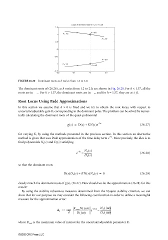
FIGURE 26.20 Dominant roots as h varies from 1.2 to 2.0.

The dominant roots of (26.26), as h varies from 1.2 to 2.0, are shown in Fig. 26.20. For h < 1.57, all the
roots are in C – . For h > 1.57, the dominant roots are in C + , and for h = 1.57, they are at ± j1.

Root Locus Using Padé Approximations
In this section we assume that h > 0 is fixed and we try to obtain the root locus, with respect to
uncertain/adjustable gain K, corresponding to the dominant poles. The problem can be solved by numer-
ically calculating the dominant roots of the quasi-polynomial

χ s() = Ds() + KN s()e −hs (26.27)

for varying K, by using the methods presented in the previous section. In this section an alternative
−hs
method is given that uses Padé approximation of the time delay term e . More precisely, the idea is to
find polynomials N h (s) and D h (s) satisfying

N h s()
−hs
e ≈ ------------- (26.28)
D h s()

so that the dominant roots

Ds()D h s() + KN s()N h s() = 0 (26.29)

closely match the dominant roots of χ(s), (26.27). How should we do the approximation (26.28) for this
match?
By using the stability robustness measures determined from the Nyquist stability criterion, we can
show that for our purpose we may consider the following cost function in order to define a meaningful
measure for the approximation error:

(
K max Njw)
(
∆ h = : sup --------------------------- e −jhw – N h jw)
------------------
(
w Djw) D h jw( )
where K max is the maximum value of interest for the uncertain/adjustable parameter K.

©2002 CRC Press LLC