Page 835 - The Mechatronics Handbook

066_Frame_C26 Page 20 Wednesday, January 9, 2002 1:59 PM

Step 2. Construct the polynomial A i (x) according to

A i x() : D s i + x)D s i – x) e −2hs i N s i + x)N s i – x)
(
(
(
(
=
–
Step 3. For each imaginary axis roots x of A i , perform the following test:
Check if |χ(σ i + x )| = 0; if yes, then r = σ i + x is a root of χ(s); if not, discard x .
Step 4. If i = M, stop; else increase i by 1 and go to Step 2.
Example
We will find the dominant roots of

−hs
1 + e -------- = 0 (26.26)
s

for a set of critical values of h. Recall that (26.26) has a pair of roots ± j1 when h = π/2 = 1.57. Moreover,
dominant roots of (26.26) are in the right half plane if h > 1.57, and they are in the left half plane if h <
∈
1.57. So, it is expected that for h (1.2, 2.0) the dominant roots are near the imaginary axis. Take σ min =
−0.5 and σ max = 0.5, with M = 400 linearly spaced σ i ’s between them. In this case

2
A i x() = s i – e −2hs i – x 2
−2hs 2
Whenever e i ≥ s i , A i (x) has two roots:

x = ± je −2hs i – s i , = 1, 2
2

For each fixed σ i satisfying this condition, let r = σ i + x (note that x is a function of s i , so r is a
function of σ i ) and evaluate

−hr
() := 1 + e
f s i ----------
r
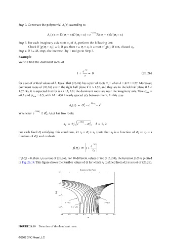
If f(σ i ) = 0, then r is a root of (26.26). For 10 different values of h (1.2, 2.0), the function f(σ) is plotted∈
in Fig. 26.19. This figure shows the feasible values of σ i for which r (defined from s i ) is a root of (26.26).

Detection of the Roots
1
10

0
10
f( σ)
10 −1

h = 1.2 h = 2.0
−2
10 h = 1.29
−0.4 −0.3 −0.2 −0.1 0 0.1 0.2 0.3
σ

FIGURE 26.19 Detection of the dominant roots.

©2002 CRC Press LLC