Page 831 - The Mechatronics Handbook

066_Frame_C26 Page 16 Wednesday, January 9, 2002 1:59 PM

26.4 Complementary Root Locus

In the previous section, the root locus parameter K was assumed to be positive and the phase and
magnitude rules were established based on this assumption. There are some situations in which controller
gain can be negative as well. Therefore, the complete picture is obtained by drawing the usual root locus
(for K > 0) and the complementary root locus (for K < 0). The complementary root locus rules are

n m
±
±
× 360° = ∑ ∠ ( rp i ) – ∑ ∠ ( rz j ), = 0, 1, 2,… (26.16)
–
–
i=1 j=1
∏ n –
K = -------------------------- (26.17)
rp i
i=1
∏ m –
j=1 rz j
Since the phase rule (26.16) is the 180° shifted version of (26.9), the complementary root locus is obtained
by simple modifications in the root locus construction rules. In particular, the number of asymptotes
and their center are the same, but their angles α ’s are given by

2
(
a = ------------------ × 180°, = 0,…, nm 1)
–
–
( nm)
–
Also, an interval on the real axis is on the complementary root locus if and only if it is not on the usual
root locus.
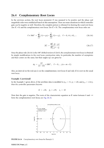
Example 3 (revisited)
In the Example 3 given above, if the problem data is modified to p m = −5, p 1 = −20, and p 2,3 = −2 ± j,
then the controller parameters become

K = – 10, p c = – 19, z c = 10

Note that the gain is negative. The roots of the characteristic equation as K varies between 0 and −∞
form the complementary root locus; see Fig. 26.16.

Complementary Root Locus
10
8 arrows indicate
increasing direction
6 of K from ∞ to 0
4
2
Imag Axis 0
−2
−4
−6
−8
−10
−25 −20 −15 −10 −5 0 5 10 15 20 25
Real Axis

FIGURE 26.16 Complementary root locus for Example 3.

©2002 CRC Press LLC