Page 828 - The Mechatronics Handbook

066_Frame_C26 Page 13 Wednesday, January 9, 2002 1:59 PM

Also note that if τ m is large, then P m (s) ≈ P b (s) , where P b (s) = K b /s 2 is the transfer function of a rigid
beam. In this example, the general class of plants P m (s) will be considered. Assuming that p m = −1/τ m and
K m are given, a first-order controller

–
Cs() = K c   sz c (26.14)
------------
– 
sp c
will be designed. The aim is to place the closed-loop system poles far from the Im-axis. Since the order
of F(s) = P m (s)C(s)/K m K c is three, the root locus has three branches. Suppose the desired closed-loop
poles are given as p 1 , p 2 , and p 3 . Then, the pole placement problem amounts to finding {K c , z c , p c } such
that the characteristic equation is
c s() = ( sp 1 ) sp 2 ) sp 3 )
(
(
–
–
–
= s – ( p 1 + p 2 + p 3 )s + ( p 1 p 2 + p 1 p 3 + p 2 p 3 )sp 1 p 2 p 3
3
2
–
But the actual characteristic equation, in terms of the unknown controller parameters, is
χ s() = ss p m ) sp c ) + ks z c )
(
(
(
–
–
–
3
2
= s – ( p m + p c )s + ( p m p c + K)sKz c
–
where K := K m K c . Equating the coefficients of the desired χ(s) to the coefficients of the actual χ(s), three
equations in three unknowns are obtained:
p m + p c = p 1 + p 2 + p 3
p m p c + K = p 1 p 2 + p 1 p 3 + p 2 p 3
Kz c = p 1 p 2 p 3
From the first equation p c is determined, then K is obtained from the second equation, and finally z c is
computed from the third equation.
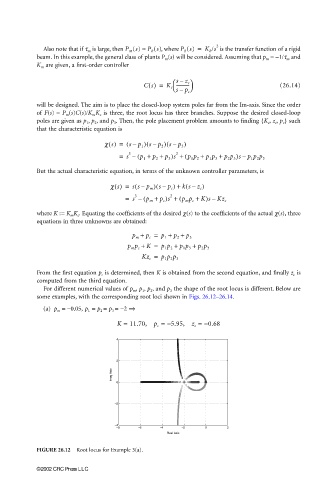
For different numerical values of p m , p 1 , p 2 , and p 3 the shape of the root locus is different. Below are
some examples, with the corresponding root loci shown in Figs. 26.12–26.14.
(a) p m = −0.05, p 1 = p 2 = p 3 = −2 ⇒

K = 11.70, p = −5.95, z = −0.68
c c

4

2
Imag Axis

0

−2

−4
−8 −6 −4 −2 0 2
Real Axis
FIGURE 26.12 Root locus for Example 3(a).

©2002 CRC Press LLC