Page 826 - The Mechatronics Handbook

066_Frame_C26 Page 11 Wednesday, January 9, 2002 1:59 PM

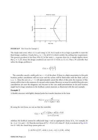
rlocus(1,[1,3,2,0])
3
2

1
Imag Axis 0

−1

−2
−3
−4 −3 −2 −1 0 1 2
Real Axis

FIGURE 26.9 Root locus for Example 1.

The steady state error, when r(t) is unit ramp, is 2/K. So K needs to be as large as possible to meet the
third design condition. Clearly, Re(r 1,2 ) = −1 for all K ≥ 1 , which satisfies the settling time requirement.
The percent overshoot is less than 10% if ζ of the roots r 1,2 is greater than 0.6. A simple algebra shows
that z = 1/ K , hence the design conditions are met if K = 1/0.36, i.e. K c = 2. Thus a PI controller that
solves the design problem is

s +

Cs() = 2 ----------- 1 

s 
The controller cancels a stable pole (at s = −1) of the plant. If there is a slight uncertainty in this pole
location, perfect cancellation will not occur and the system will be third-order with the third pole at
r 3 ≅ – 1 . Since the zero at z o = −1 will approximately cancel the effect of this pole, the response of this
system will be close to the response of a second-order system. However, we must be careful if the pole–zero
cancellations are near the imaginary axis because in this case small perturbations in the pole location
might lead to large variations in the feedback system response, as illustrated with the next example.
Example 2
A flexible structure with lightly damped poles has transfer function in the form

2
Ps() = ----------------------------------------------
w 1
2
2
(
2
s s + 2zw 1 s + w 1 )
By using the root locus, we can see that the controller
(
2
2
( s + 2zw 1 s + w 1 ) s + 0.4)
Cs() = K c ---------------------------------------------------------------
(
2
( s + r) s + 4)
stabilizes the feedback system for sufficiently large r and an appropriate choice of K c . For example, let
2
ω 1 = 2, ζ = 0.1, and r = 10. Then the root locus of F(s) = P(s)C(s)/K, where K = K c w 1 , is as shown in Fig. 26.10.
For K = 600, the closed-loop system poles are
±
±
{ – 10.78 ± j2.57, 0.94 j1.61, 0.2 j1.99, 0.56}
–
–
–
©2002 CRC Press LLC