Page 824 - The Mechatronics Handbook

066_Frame_C26 Page 9 Wednesday, January 9, 2002 1:59 PM

Im
-4+j2
∆ 1
4
5
3
-5 -3 1 Re
2
-4-j2

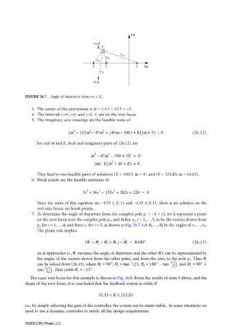
FIGURE 26.7 Angle of departure from −4 + j2.

3. The center of the asymptotes is s = (−12 + 3)/3 = −3.
4. The intervals (−∞, −5] and [−3, 1] are on the root locus.
5. The imaginary axis crossings are the feasible roots of

(
( w – j12w 47w + j40w 100) + Kjw + 3) = 0 (26.12)
4
3
2
–
–
for real ω and K. Real and imaginary parts of (26.12) are
4 2
w – 47w – 100 + 3K = 0
jw −12w + 40 + K) = 0
2
(
They lead to two feasible pairs of solutions (K = 100/3, ω = 0) and (K = 215.83, ω = ±4.62).
6. Break points are the feasible solutions of
3s + 36s + 155s + 282s + 220 = 0
3
4
2
Since the roots of this equation are −4.55 ± j1.11 and −1.45 ± j1.11, there is no solution on the
real axis, hence no break points.
7. To determine the angle of departure from the complex pole p 1 = −4 + j2, let ∆ represent a point
on the root locus near the complex pole p 1 , and define v i , i = 1,…,5, to be the vectors drawn from
p i , for i = 1,…,4, and from z 1 for i = 5, as shown in Fig. 26.7. Let θ 1 ,…,θ 5 be the angles of v 1 ,…,v 5 .
The phase rule implies

( q 1 + q 2 + q 3 + q 4 ) q 5 = ± 180° (26.13)
–

As ∆ approaches p 1 , θ 1 becomes the angle of departure and the other θ i ’s can be approximated by
the angles of the vectors drawn from the other poles, and from the zero, to the pole p 1 . Thus θ 1
can be solved from (26.13), where q 2 ≈ 90° , q 3 ≈ tan () , q 4 ≈ 180° tan – 1 2  , and q 5 ≈ 90°+
–
1
–
2
--
5 
tan – 1 1  . That yields q 1 ≈ – 15° .
--
2 
The exact root locus for this example is shown in Fig. 26.8. From the results of item 5 above, and the
shape of the root locus, it is concluded that the feedback system is stable if
33.33 < K < 215.83
i.e., by simply adjusting the gain of the controller, the system can be made stable. In some situations we
need to use a dynamic controller to satisfy all the design requirements.
©2002 CRC Press LLC