Page 819 - The Mechatronics Handbook

066_Frame_C26 Page 4 Wednesday, January 9, 2002 1:58 PM

Root Locus
2
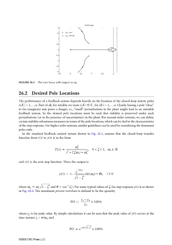
x : ω o = zero
1.5
o : ω = infinity
o
1
0.5
0
−0.5
−1
−1.5
−2
−2.5 −2 −1.5 −1 −0.5 0

FIGURE 26.3 The root locus with respect to w o .

26.2 Desired Pole Locations

The performance of a feedback system depends heavily on the location of the closed-loop system poles
r i (K) = 1,…,n. First of all, for stability we want r i (K) − for all i = 1,…,n. Clearly, having a pole “close”
to the imaginary axis poses a danger, i.e., “small” perturbations in the plant might lead to an unstable
feedback system. So the desired pole locations must be such that stability is preserved under such
perturbations (or in the presence of uncertainties) in the plant. For second-order systems, we can define
certain stability robustness measures in terms of the pole locations, which can be tied to the characteristics
of the step response. For higher order systems, similar guidelines can be used by considering the dominant
poles only.
In the standard feedback control system shown in Fig. 26.1, assume that the closed-loop transfer
function from r(t) to y(t) is in the form

2
Ts() = -------------------------------------, 0 << 1, w o ∈
w o
z
s + 2zw o s + w o 2
2
and r(t) is the unit step function. Then, the output is
−zw t
o
e
yt() = 1 ------------------sin ( w d t + θ), t ≥ 0
–
2
–
1 z
2 −1
where w d := w o 1 ζ– and θ := cos (ζ). For some typical values of ζ, the step response y(t) is as shown
in Fig. 26.4. The maximum percent overshoot is defined to be the quantity
y p – y ss
PO := ---------------- × 100%
y ss

where y p is the peak value. By simple calculations it can be seen that the peak value of y(t) occurs at the
time instant t p = π/ω d , and

2
PO = e −pz/ 1−z × 100%

©2002 CRC Press LLC