
Page 817 - The Mechatronics Handbook
P. 817
066_Frame_C26 Page 2 Wednesday, January 9, 2002 1:58 PM
v(t)
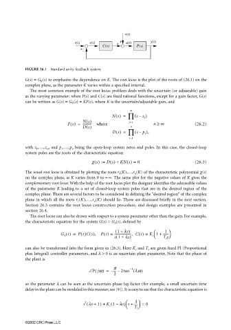
r(t) e(t) + + u(t) y(t)
C(s) P(s)
+
-
FIGURE 26.1 Standard unity feedback system.
G(s) = G K (s) to emphasize the dependence on K. The root locus is the plot of the roots of (26.1) on the
complex plane, as the parameter K varies within a specified interval.
The most common example of the root locus problem deals with the uncertain (or adjustable) gain
as the varying parameter: when P(s) and C(s) are fixed rational functions, except for a gain factor, G(s)
can be written as G(s) = G K (s) = KF(s), where K is the uncertain/adjustable gain, and
m
Ns() = ∏ ( sz j )
–
Fs() = Ns() where j=1 n ≥ m (26.2)
-----------
Ds() n
Ds() = ∏ ( sp i ),
–
i=1
with z 1 ,…,z m , and p 1 ,…,p n being the open-loop system zeros and poles. In this case, the closed-loop
system poles are the roots of the characteristic equation
c s() : Ds() + KN s() = 0 (26.3)
=
The usual root locus is obtained by plotting the roots r 1 (K),…,r n (K) of the characteristic polynomial χ(s)
on the complex plane, as K varies from 0 to +∞. The same plot for the negative values of K gives the
complementary root locus. With the help of the root locus plot the designer identifies the admissible values
of the parameter K leading to a set of closed-loop system poles that are in the desired region of the
complex plane. There are several factors to be considered in defining the “desired region” of the complex
plane in which all the roots r 1 (K),…,r n (K) should lie. Those are discussed briefly in the next section.
Section 26.3 contains the root locus construction procedure, and design examples are presented in
section 26.4.
The root locus can also be drawn with respect to a system parameter other than the gain. For example,
the characteristic equation for the system G(s) = G λ (s), defined by
( 1 ls) 1
–
G l s() = Ps()Cs(), Ps() = ---------------------, Cs() = K c 1 + -------
s 1 + ls) T I s
(
can also be transformed into the form given in (26.3). Here K c and T I are given fixed PI (Proportional
plus Integral) controller parameters, and λ > 0 is an uncertain plant parameter. Note that the phase of
the plant is
∠ Pjw) = – p 2tan −1 ( lw)
(
--- –
2
so the parameter λ can be seen as the uncertain phase lag factor (for example, a small uncertain time
delay in the plant can be modeled in this manner, see [9]). It is easy to see that the characteristic equation is
1
(
s ls + 1) + K c 1 ls) s + ----- = 0
(
2
–
T I
©2002 CRC Press LLC