Page 818 - The Mechatronics Handbook

066_Frame_C26 Page 3 Wednesday, January 9, 2002 1:58 PM

2
2
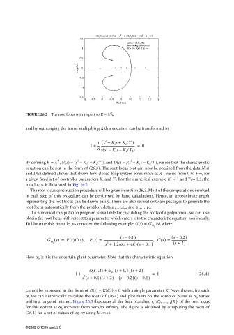
Root Locus for N(s) = s + s + 0.4, D(s) = s(s − s − 0.4)
1.5
arrows show the
increasing direction of
1 K = 1/λ from 0 to +∞
0.5
Imag Axis 0

−0.5

−1
−1.5
−2 −1.5 −1 −0.5 0 0.5 1 1.5 2
Real Axis

FIGURE 26.2 The root locus with respect to K = 1/l.

and by rearranging the terms multiplying λ this equation can be transformed to

1 s +( 2 K c s + K c /T I )
1 + --- -------------------------------------------- = 0
l ss – K c s K c /T I )
(
2
–
2
−1
2
By defining K = λ , N(s) = (s + K c s + K c /T I ), and D(s) = s(s − K c s − K c /T I ), we see that the characteristic
equation can be put in the form of (26.3). The root locus plot can now be obtained from the data N(s)
−1
and D(s) defined above; that shows how closed-loop system poles move as λ varies from 0 to +∞, for
a given fixed set of controller parameters K c and T I . For the numerical example K c = 1 and T I = 2.5, the
root locus is illustrated in Fig. 26.2.
The root locus construction procedure will be given in section 26.3. Most of the computations involved
in each step of this procedure can be performed by hand calculations. Hence, an approximate graph
representing the root locus can be drawn easily. There are also several software packages to generate the
root locus automatically from the problem data z 1 ,…,z m , and p 1 ,…,p n .
If a numerical computation program is available for calculating the roots of a polynomial, we can also
obtain the root locus with respect to a parameter which enters into the characteristic equation nonlinearly.
(s) where
To illustrate this point let us consider the following example: G(s) = G w
o
( s 0.1) ( s 0.2)
–
–
G w s() = Ps()Cs(), Ps() = ----------------------------------------------------------------, Cs() = -------------------
(
2
2
o ( s + 1.2w o s + w o ) s + 0.1) ( s + 2)
Here ω o ≥ 0 is the uncertain plant parameter. Note that the characteristic equation
w o 1.2s +( w o ) s + 0.1) s + 2)
(
(
1 + --------------------------------------------------------------------------------------- = 0 (26.4)
(
(
s s + 0.1) s + 2) + ( s 0.2) s 0.1)
(
2
–
–
cannot be expressed in the form of D(s) + KN(s) = 0 with a single parameter K. Nevertheless, for each
ω o we can numerically calculate the roots of (26.4) and plot them on the complex plane as ω o varies
within a range of interest. Figure 26.3 illustrates all the four branches, r 1 (K),…,r 4 (K), of the root locus
for this system as ω o increases from zero to infinity. The figure is obtained by computing the roots of
(26.4) for a set of values of ω o by using MATLAB.
©2002 CRC Press LLC