Page 821 - The Mechatronics Handbook

066_Frame_C26 Page 6 Wednesday, January 9, 2002 1:58 PM

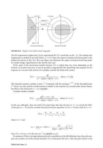
FIGURE 26.6 Region of the desired closed-loop poles.
≥
≤
The PO requirement implies that ζ 0.6, equivalently θ 53° (recall that cos(θ) = ζ). The settling time
≤
requirement is satisfied if and only if Re(r 1,2 ) −0.5. Then, the region of desired closed-loop poles is the
shaded area shown in Fig. 26.6. The same figure also illustrates the region of desired closed-loop poles
for similar design requirements in the discrete time case.
If the order of the closed-loop transfer function T(s) is higher than two, then, depending on the
location of its poles and zeros, it may be possible to approximate the closed-loop step response by the
response of a second-order system. For example, consider the third-order system

2
Ts() = --------------------------------------------------------------- where r >> zw o
w o
(
2
2
( s + 2zw o s + w o ) 1 + s/r)
−zw t
o
−rt
The transient response contains a term e . Compared with the envelope e of the sinusoidal term,
−rt
e decays very fast, and the overall response is similar to the response of a second-order system. Hence,
the effect of the third pole r 3 = −r is negligible.
Consider another example,
w o 1 + s/ r + )]
(
[
2
Ts() = --------------------------------------------------------------- where 0 < << r
2
(
2
( s + 2zw o s + w o ) 1 + s/r)
In this case, although r does not need to be much larger than ζω o , the zero at −(r + ) cancels the effect
of the pole at −r. To see this, consider the partial fraction expansion of Y(s) = T(s)R(s) with R(s) = 1/s:
A 1
A 3
A 0
Ys() = ----- + ------------ + ------------ + ----------
A 2
–
s sr 1 sr 2 s + r
–
where A 0 = 1 and
2


A 3 = lim ( s + r)Ys() = ------------------------------------------ ----------- 
w o
2 

2
s→ −r 2zw o r ( w o + r ) r + 
–
Since A 3 → 0 as → 0 , the term A 3 e is negligible in y(t).
−rt
In summary, if there is an approximate pole–zero cancellation in the left half plane, then this pole–zero
pair can be taken out of the transfer function T(s) to determine PO and t s . Also, the poles closest to the
©2002 CRC Press LLC