Page 832 - The Mechatronics Handbook

066_Frame_C26 Page 17 Wednesday, January 9, 2002 1:59 PM

Complete Root Locus for −∞ < K < +∞
5
4
3
2
1
Imag Axis 0
−1
−2
−3
−4
−5
−4 −2 0 2 4 6 8
Real Axis

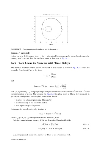
FIGURE 26.17 Complementary and usual root loci for Example 4.
Example 4 (revisited)
In this example, if K increases from ∞ to +∞ , the closed-loop system poles move along the comple-
–
mentary root locus, and then the usual root locus, as illustrated in Fig. 26.17.
26.5 Root Locus for Systems with Time Delays

The standard feedback control system considered in this section is shown in Fig. 26.18, where the
controller C and plant P are in the form
N c s()
Cs() = -------------
D c s()

and
N p s()
hs
–
Ps() = e P 0 s() where P 0 s() = -------------
D p s()
2
−hs
with (N c , D c ) and (N p , D p ) being coprime pairs of polynomials with real coefficients. The term e is the
transfer function of a pure delay element (in Fig. 26.18 the plant input is delayed by h seconds). In
general, time delays enter into the plant model when there is
• a sensor (or actuator) processing delay, and/or
• a software delay in the controller, and/or
• a transport delay in the process.
In this case the open-loop transfer function is

Gs() = G h s() = e G 0 s()
–
hs
where G 0 (s) = P 0 (s)C(s) corresponds to the no delay case, h = 0.
Note that magnitude and phase of G( jw) are determined from the identities
(
Gjw) = G 0 jw( ) (26.18)
∠ Gjw) = – hw + ∠ G 0 jw) (26.19)
(
(
2
A pair of polynomials is said to be coprime pair if they do not have common roots.

©2002 CRC Press LLC