Page 846 - The Mechatronics Handbook

0066_frame_C27 Page 7 Wednesday, January 9, 2002 7:10 PM

due to the zero at ω = 5. Finally at ω = 10 the slope becomes −60 dB/decade due to the complex conjugate
poles at ω n = 10.
The exact magnitude is obtained by calculating the actual magnitude at important frequencies such
as the corner or natural frequencies of each factor. The phase curve can be obtained by adding the phase
due to each factor. Although the linear approximation of the phase characteristic for a single pole or zero
is suitable for initial analysis, the error between the exact phase curve and the linear approximation of
complex conjugate poles can be large, as seen in Fig. 27.6. Hence, if the accurate phase angle curve is
required, a computer program such as Matlab or Ctrl-C can be utilized to generate the actual phase curve.

27.3 Polar Plots

The polar plot of a sinusoidal transfer function G(jω) is a plot of both the magnitude and the phase of
the frequency response in polar coordinates as the frequency ω varies from zero to infinity. Since the
sinusoidal transfer function G(jω) can be expressed as

(
Gjw) = Re Gjw)] + j Im Gjw)] = Gjw) e jf
(
[
(
(
[
the polar plot of G(jω) is a plot of Re[G(jω)] on the horizontal axis versus Im[G(jω)] on the vertical
axis in the complex G(s)-plane as ω varies from zero to infinity. Hence, for each value of ω, a polar plot
of G(jω) is defined by a vector of length |G(jω)| and a phase angle f = ∠ G(jw) , as in Eq. (27.8).
We can investigate the general shapes of polar plots according to the system types and relative degrees
of transfer functions. Relative degree of a transfer function is defined as the difference between the degree
of the denominator polynomial and that of the numerator. Consider a transfer function of the form
K 1 + jwt a ) 1 + jwt b ) …
(
(
(
Gjw) = -----------------------------------------------------------------------
(
( jw) 1 + jwt 1 ) 1 + jwt 2 ) …
(
N
(
m
b 0 jw) + b 1 jw) m−1 + …
(
= ---------------------------------------------------------------
(
a 0 jw) + b 1 jw) n−1 + …
n
(
where K > 0 and the relative degree n − m ≥ 0. The magnitudes and phase angles of G(jω) as ω approaches
zero and infinity are presented in Table 27.2. The general shapes of the polar plots of various system
types in the low-frequency portion are shown in Fig. 27.7. The high-frequency portions of the polar
plots of various relative degrees are shown in Fig. 27.8. It can be seen that the G(jω) loci are parallel to
either the horizontal or the vertical axes with infinite magnitude as w → 0 + for system types greater than
zero. If the relative degree is greater than zero, the G(jω) loci converge to the origin clockwise and are
tangent to one or the other axes. Note that the polar plot curves can be very complicated due to the
numerator and denominator dynamics over the intermediate frequency range. Therefore, the polar plot
of G(jω) in the frequency range of interest must be accurately determined.
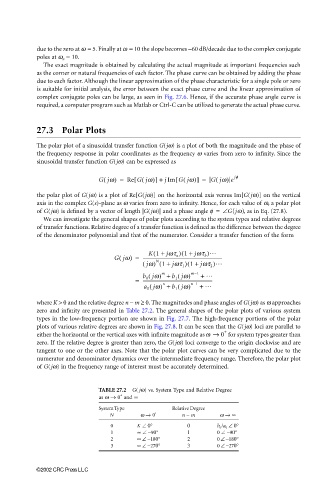
TABLE 27.2 G( jω) vs. System Type and Relative Degree
+
as ω → 0 and ∞
System Type Relative Degree
+
N ω → 0 n − m ω → ∞
0 K ∠ 0° 0 b 0 /a 0 ∠ 0°
1 ∞ ∠ −90° 1 0 ∠ −90°
2 ∞ ∠ −180° 2 0 ∠ −180°
3 ∞ ∠ −270° 3 0 ∠ −270°

©2002 CRC Press LLC