Page 849 - The Mechatronics Handbook

0066_frame_C27 Page 10 Wednesday, January 9, 2002 7:10 PM

20 10
1
G(jw) =
(1+ jwT ) (1+ jwT ) (1+ jwT )
1 2 3
10 0
jwT
G(jw) =
1+ jwT ω = 0
Gain (dB) 0 ω = 0 Gain (dB) −10

−10 −20
ω
ω
∞
∞
−20 −30
−180 −90 0 90 180 −270 −180 −90 0 90
Phase (deg)
Phase (deg)
20
0
w
0

Gain (dB) −20

2
w
n
G(jw) =
−40
2
j ω [( jω) + 2ζωn ( jω) + ωn ] 2
ω
∞
−60
−270 −180 −90 0 90
Phase (deg)
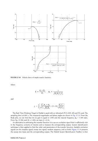
FIGURE 27.10 Nichols charts of simple transfer functions.
where

R 1 + 1
K = -----------------, w n = ------------------------------
R 2
R 2
R A R B C A C B
and

R A +
V = 1 ------------------------ + ( 1 K) -------------
R A C A
R B
C B
--
–
2 C A R A R B R B C B
The Real-Time Windows Target in Matlab is used with an Advantech PCL-818L AD and DA card. The
sampling time is 0.001 s. The measured magnitudes and phase angles are shown in Fig. 27.13. From the
Bode plot, we can find that the dc gain is equal to 1.995 and the natural frequency ω n = 17.90 rad/s.
From Eq. (27.9b) and M r = 1.993, we have ζ = 0.26.
An alternative to estimating the transfer function is to use an excitation signal that is sufficiently rich
in the frequency contents of interest and to measure the corresponding output. System identification
technique is then applied to find the order and parameters of the transfer function. Suitable excitation
signals are the impulse signal, sweep sine signal, random sequence, and so forth. Figure 27.14 presents
the sweep sine input and the corresponding output. The Matlab System Identification Toolbox is then

©2002 CRC Press LLC