Page 853 - The Mechatronics Handbook

0066_frame_C27 Page 14 Wednesday, January 9, 2002 7:10 PM

Im F(s)-plane
3
Γ 1.99
2
Γ
2.5
1
Γ Γ Γ
3.5 0.5 4.5
0
Re
−1

−2
−3
−4 −3 −2 −1 0 1 2 3

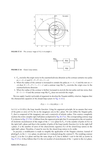
FIGURE 27.15 The contour maps of F(s) in Example 3.

FIGURE 27.16 Closed-loop system.

3. Γ 2.5 encircles the origin twice in the counterclockwise direction as the contour contains two poles
at s = −1, −2 and N = Z − P = 0 − 2 = −2.
4. When the radius of the contour is increased to contain the poles at s = −1, −2 and the zero at s =
−3, then N = Z − P = 1 − 2 = −1 and a contour map like Γ 3.5 encircles the origin once in the
counterclockwise direction.
5. When the radius of the contour is further increased to encircle the two poles and two zeros, then
N = 2 − 2 = 0 and the contour map like Γ 4.5 does not encircle the origin.
We now apply Cauchy’s principle of argument to develop the Nyquist stability criterion. Suppose that
the characteristic equation of the closed-loop system in Fig. 27.16 is

Fs() = 1 + Gs()Hs() = 0

Let L(s) = G(s)H(s), the loop transfer function. Using the argument principle, let us assume that none
of the poles or zeros of F(s) lie on the imaginary axis in the s-plane. We now define the Nyquist path,
Γ s , that is composed of the imaginary axis and a semicircle of infinite radius. This contour completely
encloses the entire complex right-half plane as depicted in Fig. 20.17(a). The corresponding contour map
Γ F is shown in Fig. 27.17(b). It follows from the argument principle that N corresponds to the net number
of clockwise encirclements of the origin of the 1 + L(s)-plane by Γ F . P is the number of poles of F(s) in
the right-half s-plane and thus is the number of poles of the loop transfer function L(s) in the right-half
s-plane. Z is the number of zeros of the characteristic equation F(s) of the closed-loop system in the
right-half s-plane. Therefore, Z must be zero for the closed-loop system to be stable.
In practice, a modification is made to simplify the application of the Nyquist criterion. Instead of
plotting Γ F in the 1 + L(s)-plane, we plot just L(s) evaluated along the contour Γ s . The resulting contour
map Γ L is in the L(s)-plane and has the same shape as Γ F but is shifted 1 unit to the left, as shown in
Fig. 27.17(c). It thus follows that N is the net number of encirclements of the −1 point in the L(s)-plane.

©2002 CRC Press LLC