Page 852 - The Mechatronics Handbook

0066_frame_C27 Page 13 Wednesday, January 9, 2002 7:10 PM

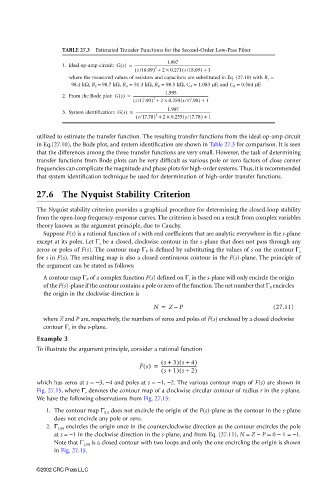
TABLE 27.3 Estimated Transfer Functions for the Second-Order Low-Pass Filter

1.997
1. Ideal op-amp circuit: Gs() = -------------------------------------------------------------------------------------
( s /18.09) + 2 × 0.271 s/18.09) + 1
(
2
where the measured values of resistors and capacitors are substituted in Eq. (27.10) with R 1 =
98.4 kΩ, R 2 = 98.7 kΩ, R A = 51.3 kΩ, R B = 98.5 kΩ, C A = 1.083 µF, and C B = 0.564 µF.
1.995
2. From the Bode plot: Gs() = ------------------------------------------------------------------------------------
2
( s/17.90) + 2 × 0.259 s/17.90) + 1
(
1.997
3. System identification: Gs() = ------------------------------------------------------------------------------------
( s/17.78) + 2 × 0.255 s/17.78) + 1
(
2
utilized to estimate the transfer function. The resulting transfer functions from the ideal op-amp circuit
in Eq.(27.10), the Bode plot, and system identification are shown in Table 27.3 for comparison. It is seen
that the differences among the three transfer functions are very small. However, the task of determining
transfer functions from Bode plots can be very difficult as various pole or zero factors of close corner
frequencies can complicate the magnitude and phase plots for high-order systems. Thus, it is recommended
that system identification technique be used for determination of high-order transfer functions.
27.6 The Nyquist Stability Criterion

The Nyquist stability criterion provides a graphical procedure for determining the closed-loop stability
from the open-loop frequency-response curves. The criterion is based on a result from complex variables
theory known as the argument principle, due to Cauchy.
Suppose F(s) is a rational function of s with real coefficients that are analytic everywhere in the s-plane
except at its poles. Let Γ s be a closed, clockwise contour in the s-plane that does not pass through any
zeros or poles of F(s). The contour map Γ F is defined by substituting the values of s on the contour Γ s
for s in F(s). The resulting map is also a closed continuous contour in the F(s)-plane. The principle of
the argument can be stated as follows:
A contour map Γ F of a complex function F(s) defined on Γ s in the s-plane will only encircle the origin
of the F(s)-plane if the contour contains a pole or zero of the function. The net number that Γ F encircles
the origin in the clockwise direction is
N = Z P (27.11)
–
where Z and P are, respectively, the numbers of zeros and poles of F(s) enclosed by a closed clockwise
contour Γ s in the s-plane.
Example 3
To illustrate the argument principle, consider a rational function
(
( s + 3) s + 4)
Fs() = --------------------------------
( s + 1) s + 2)
(
which has zeros at s = −3, −4 and poles at s = −1, −2. The various contour maps of F(s) are shown in
Fig. 27.15, where Γ r denotes the contour map of a clockwise circular contour of radius r in the s-plane.
We have the following observations from Fig. 27.15:
1. The contour map Γ 0.5 does not encircle the origin of the F(s)-plane as the contour in the s-plane
does not encircle any pole or zero.
2. Γ 1.99 encircles the origin once in the counterclockwise direction as the contour encircles the pole
at s = −1 in the clockwise direction in the s-plane, and from Eq. (27.11), N = Z − P = 0 − 1 = −1.
Note that Γ 1.99 is a closed contour with two loops and only the one encircling the origin is shown
in Fig. 27.15.

©2002 CRC Press LLC