Page 842 - The Mechatronics Handbook

0066_frame_C27 Page 3 Wednesday, January 9, 2002 7:10 PM

FIGURE 27.2 A first-order low-pass filter.

1.5
Transient Steady–state
response response
1

0.5 Output |G(jw)|
Amplitude (V) 0

−0.5 Input ∠ G(jw)

−1
0 1 2 3 4 5 6 7 8
Time (s)
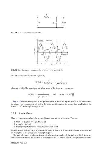
FIGURE 27.3 Frequency response of G(s) = 1/(0.5s + 1) to u(t) = sin 2t.

The sinusoidal transfer function is given by

1
1
Gjw) = ---------------------------- = -----------------------------
(
(
(
jw RC) + 1 j w /w 1 ) + 1
where ω 1 = 1/RC. The magnitude and phase angle of the frequency response are
1 w
1
Gjw) = ---------------------------------- and fw() = – tan ------
(
–
1 + ( w /w 1 ) 2 w 1
Figure 27.3 shows the response of the system with RC = 0.5 to the input u = sin2t. It can be seen that
the steady-state response is irrelevant to the initial conditions, and the steady-state amplitude of the
output is 1/ 2 and the phase angle is −45°.

27.2 Bode Plots

There are three commonly used displays of frequency response of a system. They are:
1. the Bode diagram or logarithmic plot,
2. the polar plot, and
3. the log-magnitude versus phase plot or Nichols chart.
We will present Bode diagrams of sinusoidal transfer functions in this section, followed by the sections
on polar plots and log-magnitude versus phase plots.
The main advantages in using the logarithmic plot are the capability of plotting low and high frequency
characteristics of the transfer function in one diagram, and the relative ease of adding the separate terms

©2002 CRC Press LLC