Page 879 - The Mechatronics Handbook

0066-frame-C29 Page 9 Wednesday, January 9, 2002 7:23 PM

Now consider the case where the coefficients of the filter a m = 0 for m > 1. The resulting expression
for y[n] from Eq. (29.5) would no longer be recursive since it would depend only on present and past
values of x, and not on past values of y. As a result, the impulse response would have duration N. This
type of filter is called a finite impulse response (FIR) filter. FIR filters are sometimes preferred over IIR
filters since they have linear phase in the frequency response. Linear phase means that the angle of the
frequency response is given by −θΩ, where θ is a constant. This corresponds to a delay in the time domain.
Design methods for both types of filters are described in the next two sections.

IIR Filter Design

The two methods for designing IIR filters are termed analog emulation (or indirect design) and direct
design. Analog emulation involves designing an analog filter first and then using one of the mapping
techniques described in the section “s-Plane to z-Plane Mappings” to convert it to a digital filter. This
method has advantages in that there is a wealth of design techniques for analog filters that can be used
in digital filter design. Direct design methods generally involve numerical techniques, and they are often
preferred over analog emulation when the sampling period is not very small. Direct design is beyond the
scope of this handbook; consult reference [2] for more information on the topic.
Analog filter design begins by selecting a bandwidth, a prototype of filter, and an order of the filter.
Additional specifications may be set on the amount of ripple that is allowed in the passband or stopband.
Two common analog prototypes are the Butterworth filters and the Chebyshev filters.
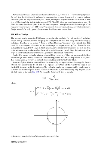
Butterworth filter: The Butterworth filter is characterized by having no zeros and having poles that are
situated on a semicircle in the left-half of the s-plane. The distance of the poles to the origin is the
bandwidth frequency and is denoted as ω b . The angle of the poles can be determined by equally spacing
out twice the number of poles around a full circle with radius ω b and then keeping only the poles in the
left-half plane, as shown in Fig. 29.5. An Nth order Butterworth filter is given by

N
Hs() = -------------------------------
w b
∏ k s w b p k )
(
–
where
–
e  jkp/N , k = N + 1 3N 1
------------- to ---------------- for N odd
 2 2
p k = 
 jk+0.5)p/N , k = N 3N 2
–
(
 e ---- to ---------------- for N even
2
2
jw

s

FIGURE 29.5 Pole distribution of a fourth-order Butterworth filter.

©2002 CRC Press LLC