Page 884 - The Mechatronics Handbook

0066-frame-C29 Page 14 Wednesday, January 9, 2002 7:23 PM

1.5

Magnitude 0.5 1

0
-3 -2 -1 0 1 2 3
Ω
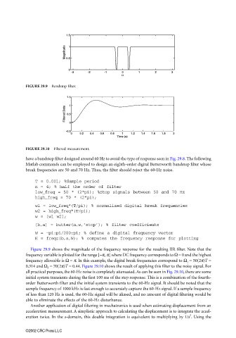
FIGURE 29.9 Bandstop filter.

1.5
1
Filtered Data 0.5

0
-0.5
0 0.2 0.4 0.6 0.8 1 1.2 1.4 1.6 1.8 2
Time (s)

FIGURE 29.10 Filtered measurement.
have a bandstop filter designed around 60 Hz to avoid the type of response seen in Fig. 29.8. The following
Matlab commands can be employed to design an eighth-order digital Butterworth bandstop filter whose
break frequencies are 50 and 70 Hz. Thus, the filter should reject the 60-Hz noise.

T = 0.001; %Sample period
n = 4; % half the order of filter
low_freq = 50 * (2*pi); %Stop signals between 50 and 70 Hz
high_freq = 70 * (2*pi);

w1 = low_freq*(T/pi); % normalized digital break frequencies
w2 = high_freq*(T/pi);
w = [w1 w2];
[b,a] = butter(n,w,‘stop’); % filter coefficients
W = -pi:pi/200:pi; % define a digital frequency vector
H = freqz(b,a,W); % computes the frequency response for plotting

Figure 29.9 shows the magnitude of the frequency response for the resulting IIR filter. Note that the
frequency variable is plotted for the range [−π, π] where DC frequency corresponds to Ω = 0 and the highest
frequency allowable is Ω = π. In this example, the digital break frequencies correspond to Ω 1 = 50(2π)T =
0.314 and Ω 2 = 70(2π)T = 0.44. Figure 29.10 shows the result of applying this filter to the noisy signal. For
all practical purposes, the 60-Hz noise is completely attenuated. As can be seen in Fig. 29.10, there are some
initial system transients during the first 100 ms of the step response. This is a combination of the fourth-
order Butterworth filter and the initial system transients to the 60-Hz signal. It should be noted that the
sample frequency of 1000 kHz is fast enough to accurately capture the 60-Hz signal. If a sample frequency
of less than 120 Hz is used, the 60-Hz signal will be aliased, and no amount of digital filtering would be
able to eliminate the effects of the 60-Hz disturbance.
Another application of digital filtering in mechatronics is used when estimating displacement from an
acceleration measurement. A simplistic approach to calculating the displacement is to integrate the accel-
2
eration twice. In the s-domain, this double integration is equivalent to multiplying by 1/s . Using the

©2002 CRC Press LLC