Page 889 - The Mechatronics Handbook

0066-frame-C29 Page 19 Wednesday, January 9, 2002 7:23 PM

10 8
Motor Position (deg) 6 4

0 2
0 0.2 0.4 0.6 0.8 1 1.2 1.4
Time (s)
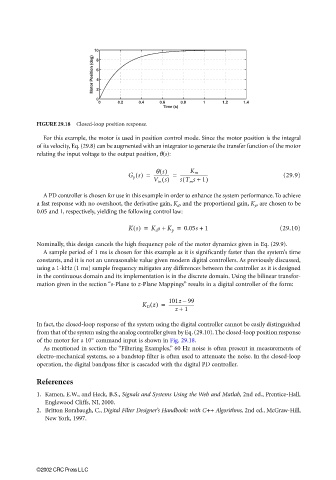
FIGURE 29.18 Closed-loop position response.

For this example, the motor is used in position control mode. Since the motor position is the integral
of its velocity, Eq. (29.8) can be augmented with an integrator to generate the transfer function of the motor
relating the input voltage to the output position, θ(s):

q s()
G p s() = -------------- = ------------------------- (29.9)
K m
V in s() sT m s + 1)
(
A PD controller is chosen for use in this example in order to enhance the system performance. To achieve
a fast response with no overshoot, the derivative gain, K d , and the proportional gain, K p , are chosen to be
0.05 and 1, respectively, yielding the following control law:
Ks() = K d s + K p = 0.05s + 1 (29.10)

Nominally, this design cancels the high frequency pole of the motor dynamics given in Eq. (29.9).
A sample period of 1 ms is chosen for this example as it is significantly faster than the system’s time
constants, and it is not an unreasonable value given modern digital controllers. As previously discussed,
using a 1-kHz (1 ms) sample frequency mitigates any differences between the controller as it is designed
in the continuous domain and its implementation is in the discrete domain. Using the bilinear transfor-
mation given in the section “s-Plane to z-Plane Mappings” results in a digital controller of the form:

–
K D z() = 101z 99
-----------------------
z + 1
In fact, the closed-loop response of the system using the digital controller cannot be easily distinguished
from that of the system using the analog controller given by Eq. (29.10). The closed-loop position response
of the motor for a 10° command input is shown in Fig. 29.18.
As mentioned in section the “Filtering Examples,” 60 Hz noise is often present in measurements of
electro-mechanical systems, so a bandstop filter is often used to attenuate the noise. In the closed-loop
operation, the digital bandpass filter is cascaded with the digital PD controller.

References

1. Kamen, E.W., and Heck, B.S., Signals and Systems Using the Web and Matlab, 2nd ed., Prentice-Hall,
Englewood Cliffs, NJ, 2000.
2. Britton Rorabaugh, C., Digital Filter Designer’s Handbook: with C++ Algorithms, 2nd ed., McGraw-Hill,
New York, 1997.

©2002 CRC Press LLC