Page 883 - The Mechatronics Handbook

0066-frame-C29 Page 13 Wednesday, January 9, 2002 7:23 PM

that are employed in data collection are also used in FIR filter design, where the modified filter is given
as h[n]w[n]. FIR design using different windows is discussed in further detail in [1,2].

Computer-Aided Design of Digital Filters
TM
Matlab is a common software package for signal processing analysis and design. The signal processing
toolbox contains several commands for designing and simulating digital filters. For example, the com-
mands butter and cheby1 automatically design a prototype analog filter for an IIR and then use the
bilinear transformation to map the filter to the discrete-time domain. Lowpass, highpass, bandstop, and
bandpass filters can be designed using these commands as long as the digital cutoff frequencies, normalized
by π, are specified. To design a digital lowpass filter based on the analog Butterworth filter with cutoff
frequency w1, use the command [b, a] = butter(N, w1∗T/pi) where N is the number of poles, T is the
sampling period, and w1∗T is digital cutoff frequency. This command puts the coefficients of the filter,
defined in Eq. (29.5), in vectors b and a in ascending order. To design a digital highpass filter with analog
cutoff frequency w1, use the commands [b, a] = butter(N, w1∗T/pi, ‘high’). To design a digital bandpass
filter with analog passband from w1 to w2, define w = [w1, w2] and use the command [b, a] = butter
(N, w ∗T/pi). To design a digital bandstop filter with stopband from w1 to w2, define w = [w1, w2] and
use the command [b, a] = butter(N, w ∗T/pi, ‘stop’). The design for an Nth order Type I Chebyshev filter
is accomplished using the same methods as for butter except that “butter” is replaced by “cheby1.”
The signal processing toolbox also provides commands for designing FIR filters. To obtain a lowpass FIR
filter with length N and analog cutoff frequency w1, use the command h = fir1(N − 1, w1∗T/pi). The
resulting vector h contains the impulse response of the FIR where h(1) is the value of h[0]. The values in
the vector h also equal the coefficients of b in Eq. (29.5) in ascending order. (Recall, that a 1 = 1 and a m = 0
for m > 1.) A length N highpass FIR filter with analog cutoff frequency w1 is designed by using the command
h = fir1(N − 1, w1∗T/pi, ‘high’). A bandpass FIR filter with passband from w1 to w2 is obtained by typing
h = fir1(N − 1, w ∗T/pi) where w = [w1, w2]. A bandstop FIR filter with stopband from w1 to w2 is obtained
by typing h = fir1(N − 1, w ∗T/pi, ‘stop’) where w = [w1, w2]. The fir1 command uses the Hamming window
by default. Other windows are obtained by adding an option of “hanning” or “boxcar” (which is the
rectangular window) to the arguments; for example, h = fir1(N − 1, w1∗T/ pi, ‘high,’ boxcar(N)) creates a
highpass FIR filter with analog cutoff frequency w1 using a rectangular window.
The filter command in Matlab is used to compute an output of a digital filter given its input sequence.
An example of its use is y = filter(b, a, x) where b and a are the coefficients of the filter and x is the input
sequence.

Filtering Examples

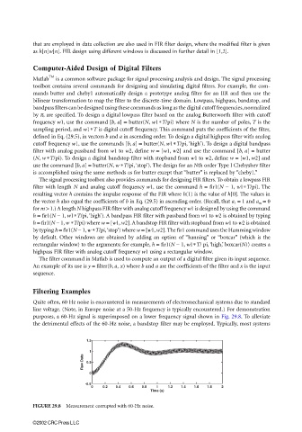
Quite often, 60 Hz noise is encountered in measurements of electromechanical systems due to standard
line voltage. (Note, in Europe noise at a 50-Hz frequency is typically encountered.) For demonstration
purposes, a 60-Hz signal is superimposed on a lower frequency signal shown in Fig. 29.8. To alleviate
the detrimental effects of the 60-Hz noise, a bandstop filter may be employed. Typically, most systems

1.5
1
Raw Data 0.5

0
-0.5
0 0.2 0.4 0.6 0.8 1 1.2 1.4 1.6 1.8 2
Time (s)
FIGURE 29.8 Measurement corrupted with 60-Hz noise.

©2002 CRC Press LLC