Page 936 - The Mechatronics Handbook

0066_Frame_C30 Page 47 Thursday, January 10, 2002 4:45 PM

Estimator (Filter) Loop Shaping
If one selects

B 1 = [ L 0 n × ] (30.260)
n
y
D 21 = [ 0 n × mIn × ] (30.261)
n
y n u y y
C 2 = C (30.262)

Θ = mI n × (30.263)
y n y
then B 1 D 21 = 0 and we have
T

T1
H f = YC 2 --- (30.264)
m

where Y ≥ 0 is the unique (at least) positive semi-definite solution of the FARE:

T T T – 1
YA + AY + LL – YC Θ CY = 0 (30.265)
Given this, the following KFDE may be derived from the FARE:

1
1
(
[
(
(
[ I + G KF jw)] I + G KF jw)] H = I + -------G FOL jw( ) -------G FOL jw) H (30.266)
m m
where
(
G FOL = CsI A) L (30.267)
−1
–
(
G KF = CsI A) H f (30.268)
−1
–
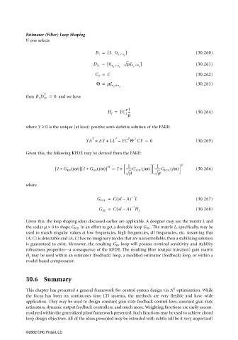
Given this, the loop shaping ideas discussed earlier are applicable. A designer may use the matrix L and
the scalar µ > 0 to shape G FOL in an effort to get a desirable loop G KF . The matrix L, specifically, may be
used to match singular values at low frequencies, high frequencies, all frequencies, etc. Assuming that
(A, C) is detectable and (A, L) has no imaginary modes that are uncontrollable, then a stabilizing solution
is guaranteed to exist. Moreover, the resulting G KF loop will possess nominal sensitivity and stability
robustness properties—a consequence of the KFDE. The resulting filter (output injection) gain matrix
H f may be used within an estimator (feedback) loop, a modified estimator (feedback) loop, or within a
model-based compensator.

30.6 Summary
2
This chapter has presented a general framework for control system design via H optimization. While
the focus has been on continuous time LTI systems, the methods are very flexible and have wide
application. They may be used to design constant gain state feedback control laws, constant gain state
estimators, dynamic output feedback controllers, and much more. Weighting functions are easily accom-
modated within the generalized plant framework presented. Such functions may be used to achieve closed
loop design objectives. All of the ideas presented may be extended with subtle (all be it very important)

©2002 CRC Press LLC