Page 935 - The Mechatronics Handbook

0066_Frame_C30 Page 46 Thursday, January 10, 2002 4:45 PM

30.5 HH 2 Output Injection Problem

This section shows how the methods presented for output feedback may be readily adopted to permit
2
the design of H optimal state estimators (filter gain matrices H f ) as well.
Generalized Plant Structure for Output Injection

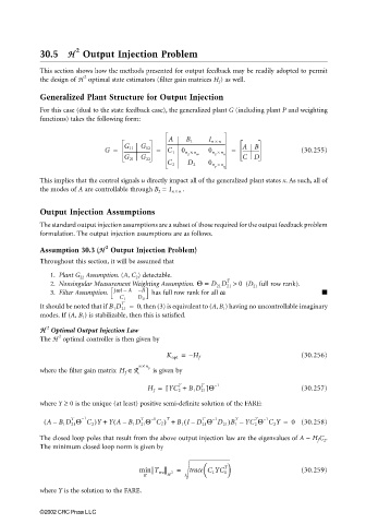
For this case (dual to the state feedback case), the generalized plant G (including plant P and weighting
functions) takes the following form:

A B 1 I n × n
G = G 11 G 12 = C 1 0 n × 0 n × = A B (30.255)
z n w z n u
G 21 G 22 CD
C 2 D 2 0 n × n
y u
This implies that the control signals u directly impact all of the generalized plant states x. As such, all of
the modes of A are controllable through B 2 = I n × n .

Output Injection Assumptions
The standard output injection assumptions are a subset of those required for the output feedback problem
formulation. The output injection assumptions are as follows.
2
Assumption 30.3 (HH Output Injection Problem)
Throughout this section, it will be assumed that
1. Plant G 22 Assumption. (A, C 2 ) detectable.
T
2. Nonsingular Measurement Weighting Assumption. Θ = D 21 D 21 > 0 (D 21 full row rank).
3. Filter Assumption. jwI – A – B has full row rank for all ω.
C 1 D 21
It should be noted that if B 1 D 21 = 0 , then (3) is equivalent to (A, B 1 ) having no uncontrollable imaginary
T
modes. If (A, B 1 ) is stabilizable, then this is satisfied.
HH 2 Optimal Output Injection Law
2
The H optimal controller is then given by
K opt = – H f (30.256)
n × n
where the filter gain matrix H f ∈ R y is given by
H f = [ YC 2 + B 1 D 21 ]Θ – 1 (30.257)
T
T
where Y ≥ 0 is the unique (at least) positive semi-definite solution of the FARE:

1
–
(
T
( AB 1 D 21 Θ C 2 )Y + Y A B 1 D 21 Θ C 2) + B 1 ID 21 Θ D 21 )B 1 – YC 2 Θ C 2 Y = 0 (30.258)
1
–
T
T
–
1
1
(
–
T
T
T
–
–
–
The closed loop poles that result from the above output injection law are the eigenvalues of A − H f C 2 .
The minimum closed loop norm is given by
 T 

min T wz 2 = trace C 1 YC 1  (30.259)
K H
where Y is the solution to the FARE.
©2002 CRC Press LLC