Page 94 - The Mechatronics Handbook

0066_Frame_C07 Page 4 Wednesday, January 9, 2002 3:39 PM

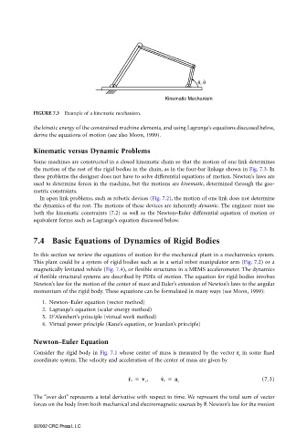
FIGURE 7.3 Example of a kinematic mechanism.

the kinetic energy of the constrained machine elements, and using Lagrange’s equations discussed below,
derive the equations of motion (see also Moon, 1999).

Kinematic versus Dynamic Problems
Some machines are constructed in a closed kinematic chain so that the motion of one link determines
the motion of the rest of the rigid bodies in the chain, as in the four-bar linkage shown in Fig. 7.3. In
these problems the designer does not have to solve differential equations of motion. Newton’s laws are
used to determine forces in the machine, but the motions are kinematic, determined through the geo-
metric constraints.
In open link problems, such as robotic devices (Fig. 7.2), the motion of one link does not determine
the dynamics of the rest. The motions of these devices are inherently dynamic. The engineer must use
both the kinematic constraints (7.2) as well as the Newton–Euler differential equation of motion or
equivalent forms such as Lagrange’s equation discussed below.

7.4 Basic Equations of Dynamics of Rigid Bodies

In this section we review the equations of motion for the mechanical plant in a mechatronics system.
This plant could be a system of rigid bodies such as in a serial robot manipulator arm (Fig. 7.2) or a
magnetically levitated vehicle (Fig. 7.4), or flexible structures in a MEMS accelerometer. The dynamics
of flexible structural systems are described by PDEs of motion. The equation for rigid bodies involves
Newton’s law for the motion of the center of mass and Euler’s extension of Newton’s laws to the angular
momentum of the rigid body. These equations can be formulated in many ways (see Moon, 1999):
1. Newton–Euler equation (vector method)
2. Lagrange’s equation (scalar-energy method)
3. D’Alembert’s principle (virtual work method)
4. Virtual power principle (Kane’s equation, or Jourdan’s principle)

Newton–Euler Equation
Consider the rigid body in Fig. 7.1 whose center of mass is measured by the vector r c in some fixed
coordinate system. The velocity and acceleration of the center of mass are given by

r ˙ c = v c , v ˙ c = a c (7.3)

The “over dot” represents a total derivative with respect to time. We represent the total sum of vector
forces on the body from both mechanical and electromagnetic sources by F. Newton’s law for the motion

©2002 CRC Press LLC