Page 98 - The Mechatronics Handbook

0066_Frame_C07 Page 8 Wednesday, January 9, 2002 3:39 PM

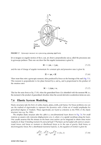
FIGURE 7.7 Gyroscopic moment on a precessing, spinning rigid body.

let us imagine an angular motion of the e 1 axis, y about a perpendicular axis e z called the precession axis
in gyroscope parlance. Then one can show that the angular momentum is given by

H = I 1 fe 1 + I z ye z (7.15)

and the rate of change of angular momentum for constant spin and presession rates is given by
˙
˙
H = ye z × H (7.16)
There must then exist a gyroscopic moment, often produced by forces on the bearings of the axel (Fig. 7.7).
This moment is perpendicular to the plane formed by e 1 and e z , and is proportional to the product of
the rotation rates:
M = I 1 fye z × e 1 (7.17)

This has the same form as Eq. (7.10), when the generalized force Q is identified with the moment M, i.e.,
the moment is the product of generalized velocities when the second derivative acceleration terms are zero.

7.6 Elastic System Modeling

Elastic structures take the form of cables, beams, plates, shells, and frames. For linear problems one can
use the method of eigenmodes to represent the dynamics with a finite set of modal amplitudes for
generalized degrees of freedom. These eigenmodes are found as solutions to the PDEs of the elastic
structure (see, e.g., Yu, 1996).
The simplest elastic structure after the cable is a one-dimensional beam shown in Fig. 7.8. For small
motions we assume only transverse displacements w(x, t), where x is a spatial coordinate along the beam.
One usually assumes that the stresses on the beam cross section can be integrated to obtain stress vector
resultants of shear V, bending moment M, and axial load T. The beam can be loaded with point or concen-
trated forces, end forces or moment or distributed forces as in the case of gravity, fluid forces, or
electromagnetic forces. For a distributed transverse load f(x, t), the equation of motion is given by

4
2
2
∂ w ∂ w ∂ w
(
D--------- – T--------- + rA--------- = fx, t) (7.18)
4
2
2
∂x ∂x ∂t
©2002 CRC Press LLC