Page 981 - The Mechatronics Handbook

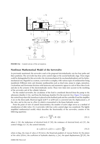
FIGURE 33.6
Control scheme of the servosystem.
Nonlinear Mathematical Model of the Servovalve
As previously mentioned, the servovalve used at the proposed electrohydraulic axis has four paths and
three positions. The servovalve has four active control edges at the second hydraulic stage. Three stages
could be distinguished by this servovalve: the electromechanical, the mechanohydraulical, and the hydro-
mechanical one. Regarded as a system, a servovalve is complex, with various types of nonlinearities being
manifested. Different static and dynamic nonlinearities such as dead zone, jump in origin, saturation,
Coulombian and Newtonian frictions with hysteresis, and asymmetry appear in each of these three levels
and also in the actuator of the electrohydraulic motor. These were taken into account in the modeling
of the servovalve and of the cylinder behavior.
For the studied servovalve, the circulation of the fluid is considered directed from the pump to the
admission chamber A (Q A ) and from the discharge chamber B to the reservoir (Q B ). Figure 33.6 presents
the control loop where the transducer is placed on the feedback path and the controller R and the amplifier
A are on the direct path. Electrical signal (±10 V or ±300 mA) is converted into the displacement x v of
the valve, and in this way in a flow Q, which is transmitted to the linear hydraulic motor.
From the point of view of control characteristics, the number of active edges serves as a method of
classification of slide valves [3]. A servovalve with four active control edges was considered. The lightly
simplified mathematical model, which describes the functionality of the servovalve, consists of the
following equations:

d t()
.
ut() = L . ----------- + R it() (33.1)
dt
where L [H], the inductance of electrical level; R [W], the resistance of electrical level; u(t) [V], the
control voltage; i(t) [A], the control intensity.

m . x v t() d . x v t() c . x v t() =+ + ∑ F (33.2)

where m [kg], the mass of valve; d [N/(m/s)], the linearized gradient of viscous friction for the piston
of the valve; c[N/m], the coefficient of hydraulic elasticity; x v [m], the spool displacement; ∑F [N], the

©2002 CRC Press LLC