Page 982 - The Mechatronics Handbook

0066_frame_Ch33.fm Page 6 Wednesday, January 9, 2002 8:00 PM

U ref + F/m .. . + x .
2
−
Σ e K UI I K IF F w 0 /c + Σ x v x v − vmax x v + x vmax
− − −
2
2D w
v 0v
w 2
0v
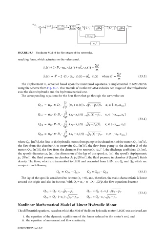
FIGURE 33.7 Nonlinear MM of the first stages of the servovalve.

resulting force, which actuates on the valve spool.
x ˙˙ v t() + 2 D v w 0v x ˙ v t() + w 0v x v t() = ∑F
.
2
.
.
.
-------
m
∗ 2 ∗ ∑F
.
.
.
.
x ˙˙ v t() = k – 2 D v w 0v x ˙ v t() w 0v x v t() where k = ------- (33.3)
–
m
The displacement x v , obtained based upon the mentioned equations, is implemented in SIMULINK
using the scheme from Fig. 33.7. This module of nonlinear MM includes two stages of electrohydraulic
axis: the electrohydraulic and the hydromechanical one.
The corresponding equations for the four flows that go through the servovalve are
2
Q PA = a D p D v . --- ( x 0 + x v t()) . p P – p A t(), x v ∈ – [ x 0 , x max ]
.
. .
r
--- (
Q AT = a D p D v . 2 . x 0 x v t()) . p A t() p T , x v ∈ – [ x max , x 0 ]
. .
–
–
r
(33.4)
Q PB = a D p D v . 2 . x 0 x v t()) . p P – p B t(), x v ∈ – [ x max , x 0 ]
--- (
. .
–
r
--- . x 0 +
Q BT = a D p D v . 2 ( x v t()) . p B t() p T , x v ∈ – [ x 0 , x max ]
. .
–
r
3
3
where Q PA [m /s], the flow to the hydraulic motor, from pump to the chamber A of the motor; Q AT [m /s],
3
the flow from the chamber A to reservoir; Q PB [m /s], the flow from pump to the chamber B of the
3
motor; Q BT [m /s], the flow from the chamber B to reservoir; α D [-], the discharge coefficient; D v [m],
the spool’s diameter; x 0 [m], the dimension of the lap of the spool; x v [m], the spool’s displacement;
3
2
2
p A [N/m ], the fluid pressure in chamber A; p B [N/m ], the fluid pressure in chamber B [kg/m ] fluids
density. The flows, which are transmitted to LHM and evacuated from LHM, are Q A and Q B , which are
computed as following:
Q A = Q PA – Q AT , Q B = Q BT – Q PB (33.5)
The lap of the spool is considered to be zero (x 0 = 0), and, therefore, the static characteristic is linear
around the origin and also in the rest. With Q 0 = α D ⋅ π ⋅ D v ⋅ 2/r , the flow equations become
Q PA = . . p P – p A , Q AT = Q 0 ( – x v ) . p A –
.
p T
Q 0 x v
(33.6)
Q PB = Q 0 ( – x v ) . p P – p B , Q BT = Q 0 x v . p B – p T
.
.
Nonlinear Mathematical Model of Linear Hydraulic Motor
The differential equations, based on which the MM of the linear hydraulic motor (LHM) was achieved, are
i. the equation of the dynamic equilibrium of the forces reduced to the motor’s rod, and
ii. the equation of movement and flow continuity.
©2002 CRC Press LLC