Page 995 - The Mechatronics Handbook

0066_frame_Ch33.fm Page 19 Wednesday, January 9, 2002 8:00 PM

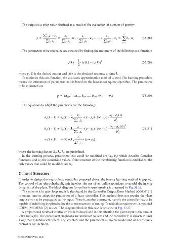
The output is a crisp value obtained as a result of the evaluation of a center of gravity:

n ⋅ n
z n
z 2
z 1
----------------------- =
y = ∑ i=1 z i w i ------------- w 1 +⋅ ------------- w 2 +⋅ … + ------------- . w n ∑ z i w i (33.28)
=
⋅
n n n n
∑ i=1 z i ∑ i=1 z i ∑ i=1 z i ∑ i=1 z i
i=1
The parameters to be estimated are obtained by finding the minimum of the following cost function:
Jk() = 1 ( yk() y d k()) 2 (33.29)
-- .
–
2
where y d (k) is the desired output and y(k) is the obtained response at time k.
To minimize this cost function, the stochastic approximation method is used. The learning procedure
means the estimation of parameters and is based on the least-mean square algorithm. The parameters
to be estimated are

p = ( a 11 ,…, a nm b 11 … b nm w 1 … w n ) (33.30)
,
,
,
,
,
,
The equations to adapt the parameters are the following:
x j – a ji t()
(
(
(
a ji t + 1) = a ji t() λλ λλ -------------- . yy d ) . w i – y) . ----------------------
z i
–
–
a
n
2
∑ l=1 z 1 b ji
( x j – a ji t()) 2
(
b ji t +( 1) = b ji t() λλ λλ -------------- . ( yy d ) . w i – y) ----------------------------- (33.31)
z i
.
–
–
b
3
n
∑ l=1 z 1 b ji
w i t + 1) = w i t() λλ λλ -------------- . ( yy d )
(
z i
–
–
w
n
∑ l=1 z 1
where the learning factors λ a , λ b , λ w are predefined.
In the learning process, parameters that could be modified are (a ji , b ji ) which describe Gaussian
functions, and w i , the conclusion values. If the structure of the membership function is established, the
only values that could be modified are w i .
Control Structure
In order to design the neuro-fuzzy controller proposed above, the inverse learning method is applied.
The control of an electrohydraulic axis involves the use of an online technique to model the inverse
dynamics of the plant. The block diagram for online inverse learning is presented in Fig. 33.26.
This scheme is in open loop and it is also found by the Controller Output Error Method (COEM) [1]
to online tune or adapt the parameters of a fuzzy controller. This method does not require the plant
output error to be propagated at the input. There is another constraint, namely the controller has to be
capable of stabilizing the plant before the commencement of tuning. To avoid this requirement, a modified
COEM (MCOEM) [2] is used. The diagram block in this case is depicted in Fig. 33.27.
A proportional feedback controller P is introduced and in this situation the plant input is the sum of
u′(k) and u p (k). The consequent singletons are initialized to zero and the controller P is chosen in such
a way that it stabilizes the plant. The structure and the parameters of inverse model and of neuro-fuzzy
controller are identical.
©2002 CRC Press LLC