Page 996 - The Mechatronics Handbook

0066_frame_Ch33.fm Page 20 Wednesday, January 9, 2002 8:00 PM

r(k)
Neuro-fuzzy u(k) y(k + 1)
y(k) Plant
controller
+
e u
Σ
− ^
u(k) y(k + 1)
Inverse model
y(k)
FIGURE 33.26 Diagram of control based on inverse learning.

r(k) u(k)
Neural Electro- y(k + 1)
y(k) Σ
controller + hydraulic axis
+
+
+ e u
u (k) Σ
p
Σ P − ^
− u(k) y(k + 1)
Inverse model y(k)

FIGURE 33.27 Block diagram for inverse learning with proportional controller.

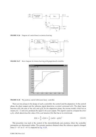
FIGURE 33.28 The position control with neuro-fuzzy controller.
There are two phases in the design of such a controller: the control and the adaptation. In the control
phase, the plant output and the reference signal determine a control command u(k). The plant input
becomes u(k), the sum of the u(k) and u p (k). In the adaptation phase, the inverse model, which has as
u ˆ
inputs y(k + 1) and y(k), produces the signal (k) as an output. This signal is used to compute the error
e u (k), which determines the value of the cost function J(k) that has to be minimized.

Jk() = 1 . 2 1 ( uk() – u ˆ k()) 2 (33.32)
-- e u k() =
-- .
2 2
This procedure was used at the control of the electrohydraulic axis position, where the controller
parameters are determined online. The actuator position obtained when the reference signal is changed
from U = 4 V to U = 8 V is depicted in Fig. 33.28.

©2002 CRC Press LLC