Page 325 - Thermal Hydraulics Aspects of Liquid Metal Cooled Nuclear Reactors

Simulation of flow-induced vibrations in tube bundles using URANS 295

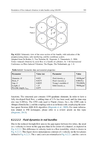
Fig. 6.2.2.1 Schematic view of the cross section of the bundle, with indication of the
postprocessing planes, tube numbering, and the coordinate system.
Adapted from De Ridder, J., Van Tichelen, K., Degroote, J., Vierendeels, J., 2016.
Vortex-induced vibrations by axial flow in a bundle of cylinders. In: 11th International
Conference on Flow-Induced Vibration, The Hague, The Netherlands, pp. 1–8.

Table 6.2.2.1 Geometric data and material properties

Parameter Value (m) Parameter Value
Diameter, D 0.025 Fluid density ρ f 1000kg/m 3
Pitch, P 0.0275 Fluid viscosity μ 0.001Pas
Gap, G 0.0025 Young’s modulus E 750,000Pa
Length, L 1.25 Solid density ρ s 7000kg/m 3
Flexible length, L flex 0.075

functions. The structural part contains 1350 quadratic elements. In order to have a
fully developed fluid flow, a settling time of 1.5s has been used, and the time-step
size was 0.289ms. The CFD code used is Fluent (Ansys, Inc.), the CSM code is
Abaqus (Simulia Inc.), and the coupling code is an in-house code, employing the inter-
face quasi-Newton (IQN-ILS) algorithm (Degroote et al., 2009). For more informa-
tion related to FSI techniques, please refer to a review article on this topic
(Degroote, 2013).

6.2.2.2.3 Fluid dynamics in rod bundles

Due to the reduced through-flow area in the gap region between two tubes, the axial
(or z-velocity) is lower in this gap area than in the center of a channel, as depicted in
Fig. 6.2.2.2. This difference in velocity leads to a flow instability, which is shown in
Fig. 6.2.2.3. This figure shows instantaneous contours of z-velocity on the two planes
defined in Fig. 6.2.2.1. The x- and y-axis are oriented as in Fig. 6.2.2.1, and the z-axis is