Page 491 - Bird R.B. Transport phenomena

§15.5 Use of the Macroscopic Balances to Solve Unsteady-State Problems 471

where
2
= Ц-0. + R + F) ± V(l + R + F) - 4R(B + F)] (15.5-29)
±
Thus by analogy with Example 7.7-2, the fluid exit temperature may approach its final value
as a monotone increasing function (overdamped or critically damped) or with oscillations
(underdamped). The system parameters appear in the dimensionless time variable, as well as
in the parameters B, F, and R. Therefore, numerical calculations are needed to determine
whether in a particular system the temperature will oscillate or not.

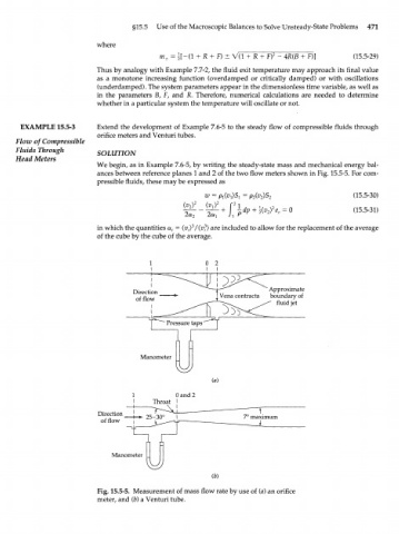
EXAMPLE 15.5-3 Extend the development of Example 7.6-5 to the steady flow of compressible fluids through
orifice meters and Venturi tubes.
Flow of Compressible
Fluids Through SOLUTION
Head Meters
We begin, as in Example 7.6-5, by writing the steady-state mass and mechanical energy bal-
ances between reference planes 1 and 2 of the two flow meters shown in Fig. 15.5-5. For com-
pressible fluids, these may be expressed as

w = (15.5-30)
(v ) 2
2
2a 2 2a, + -I (15.5-31)
3
in which the quantities a, = (^,) /(У?) are included to allow for the replacement of the average
of the cube by the cube of the average.

Approximate
boundary of
fluid jet

Manometer

(a)

0and2

Direction
of flow

Manometer

Fig. 15.5-5. Measurement of mass flow rate by use of (a) an orifice
meter, and (b) a Venturi tube.