Page 110 - Using ANSYS for Finite Element Analysis Dynamic, Probabilistic, Design and Heat Transfer Analysis

probabilistic Design analysis • 97
• The individual simulation loops are inherently independent; the
individual simulation loops do not depend on the results of any
other simulation loops. This makes Monte Carlo Simulation tech-
niques ideal candidates for parallel processing.

The Direct Sampling Monte Carlo technique has one drawback: it is
not very efficient in terms of required number of simulation loops.

3.4.1 DiReCT SAMPLing

Direct Monte Carlo Sampling is the most common and traditional form of
a Monte Carlo analysis. It is popular because it mimics natural processes
that everybody can observe or imagine and is therefore easy to understand.
For this method, you simulate how your components behave based on the
way they are built. One simulation loop represents one component that is
subjected to a particular set of loads and boundary conditions. The Direct
Monte Carlo Sampling technique is not the most efficient technique, but it is
still widely used and accepted, especially for benchmarking and validating
probabilistic results. However, benchmarking and validating requires many
simulation loops, which is not always feasible. This sampling method is
also inefficient due to the fact that the sampling process has no “memory.”
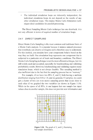
For example, if we have two RVs X and X both having a uniform
1
2
distribution ranging from 0.0 to 1.0, and we generate 15 samples, we could
get a cluster of two (or even more) sampling points that occur close to
each other if we graphed the two variables (as shown in Figure 3.10).
While in the space of all RVs, it can happen that one sample has input
values close to another sample, this does not provide new information and

1
X 2

0
0 X 1 1
Figure 3.10. The graph of X and X illustrating
2
1
bad sample distribution.