Page 41 - Using ANSYS for Finite Element Analysis A Tutorial for Engineers

28 • Using ansys for finite element analysis
1.5.2 work or energy Methods

To develop the stiffness matrix and equations for two- and three-
dimensional elements, it is much easier to apply a work or energy method.
These are based on variational calculus. The variational method is appli-
cable to problems that can be stated by certain integral expressions such
as the expression for potential energy. The principle of virtual work (using
virtual displacement), the principle of minimum potential energy, and
Castigliano’s theorem are methods frequently used for the purpose of der-
ivation of element equations. The principle of virtual work is applicable
for any material behavior, whereas the principle of minimum potential
energy and Castigliano’s theorem are applicable only to elastic materials.
For the purpose of extending, FEM outside the structural stress anal-
ysis field, a functional (a scalar function of other functions) analogous to
the one to be used with the principle of minimum potential energy is quite
useful in deriving the element stiffness matrix and equations.

1.5.3 Methods of weighted residuals

Weighted residual methods are particularly suited to problems for which
differential equations are known, but no variational statement or func-
tional is available. For stress analysis and some other problem areas, the
variational method and the most popular weighted residual method (the
Galerkin method) yield identical finite element formulations.

1.6 derivation of sPring element
eqUations Using direCt method

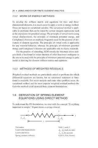
To understand the FE formulation, we start with the concept “Everything
important is simple.” Figure shows a spring element

1 k 2
x ˆ
ˆ
ƒ ,d ˆ 1x ƒ ,d ˆ 2x
ˆ
1x
2x
L
Two nodes: Node 1, node 2
ˆ
Local nodal displacements: d ˆ 1x ,d (inch, m, mm)
2x
ˆ
Local nodal forces: ƒ ˆ 1x 2x
,f (lb, newton)
Spring constant (stiffness) K (lb/in, N/m, N/mm)