Page 43 - Using ANSYS for Finite Element Analysis A Tutorial for Engineers

30 • Using ansys for finite element analysis
Apply boundary condition:

∧ ∧ ∧ ∧ ∧ ∧
u
0
At x = 0 u = d x ∴ () = a + a () = d x ∴ a = d x1
0
1
1
2
1
1
∧ ∧
∧
∧
∧
∧
∧
At x = L u = d x ∴ () = a + a () = d x ∴ a = d x − d x1
uL
2
L
2
2
2
1
L
1
Substituting values of coefficients:
 ∧ ∧   ∧ x  ∧  ∧ x  ∧  ∧ x ∧ x   ∧ 
∧

1
u ∧ +  d x2 − d x1  x ∧ =  1 − +   d x = 1 −   d x 

∴= d x1  d x1 2 
 L   L   L   L L  ∧

         d x  
2
∧
 
∧
u
N
d
∴= [] 
 
∧ ∧ x
x
Where N =− L and N = L
1
2
1
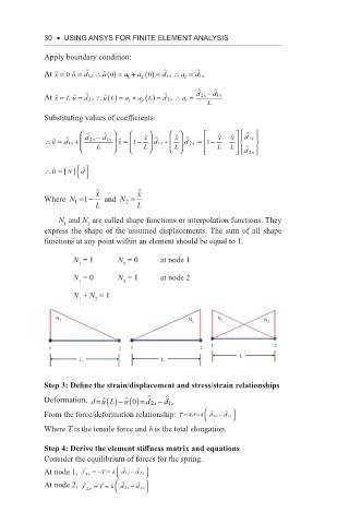
N and N are called shape functions or interpolation functions. They
2
1
express the shape of the assumed displacements. The sum of all shape
functions at any point within an element should be equal to 1.
N = 1 N = 0 at node 1
2
1
N = 0 N = 1 at node 2
2
1
N + N = 1
2
1
N 1 N 2 N 1 N 2
1 2 1 2 1 2
L
L L
Step 3: Define the strain/displacement and stress/strain relationships
∧
∧
∧
∧
Deformation, d = () − ()= d x2 − d x1
L
u
u 0
 ∧
∧
From the force/deformation relationship: Tk= d = kd x − d x   

2

1
Where T is the tensile force and δ is the total elongation.
Step 4: Derive the element stiffness matrix and equations
Consider the equilibrium of forces for the spring.
∧  ∧ ∧ 
At node 1, f 1 =− T = kd x − d x  

x
2
1

∧  ∧ ∧ 
At node 2, f = T = kd x − d x 
2 x   2 1 