Page 46 - Using ANSYS for Finite Element Analysis A Tutorial for Engineers

IntroductIon to FInIte element AnAlysIs • 33

∧ ∧
∧
∧
∧
∧
∧
uL
2
a L
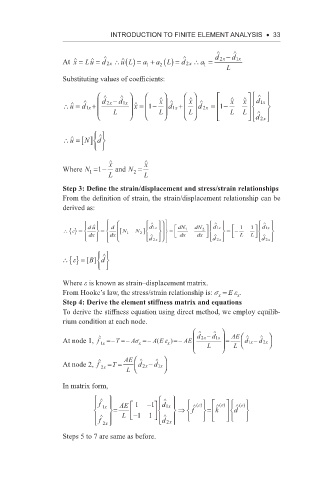
At x = Lu = d x ∴ () = a + () = d x ∴ a = d x − d x 1
2
2
1
2
1
L
Substituting values of coefficients:
 ∧ ∧   ∧ x     ∧ x ∧ x   ∧ 
∧
x
u ∧ ∧ +  d x2 − d x1  x ∧ ∧ ∧  −   d x 1 


2
∴= d x1 =  1 −  d x1 +   d x = 1
 L   L   L   L L   ∧ 
         2 
d x
 
∧
∧
u
d
N
∴= [] 
 
∧ x x ∧
1
Where N =− and N =
1
2
L L
Step 3: Define the strain/displacement and stress/strain relationships
From the definition of strain, the strain/displacement relationship can be
derived as:
 du ∧   d   ∧    ∧   ∧ 
 d 1x 
1
1
  =
 =−
e
∴{} =       [ N 1 N 2 ]  d x     dN 1 dN 2   d x    1 1  1 
 = 
 
 


∧
∧
  dx   dx    d x     dx dx    d x   L L    d ∧ 2x  

 


2
2
 
∧
∴{} = []Bd
e
 
 
Where e is known as strain–displacement matrix.
From Hooke’s law, the stress/strain relationship is: s = E e .
x
x
Step 4: Derive the element stiffness matrix and equations
To derive the stiffness equation using direct method, we employ equilib-
rium condition at each node.
 ∧ ∧ 
∧ d x2 − AE  ∧ ∧  
At node 1, f =− T =− As =− A E e ) =− AE  d x1  =  d x1 − d x2 
(
x 1 x x  L  L  
 
∧ AE  ∧ ∧ 
At node 2, f ==  d x2 − 
T
2 x L  d x1 
In matrix form,
 ∧   ∧ 


 f x 1  AE 1 − 1  d x 1    ∧()  ∧()  ∧() 



e
e
e
  =     ⇒  f  = k   d 
 f ∧  L  − 1 1   ∧             
 2 x   d x 
2
Steps 5 to 7 are same as before.