Page 44 - Using ANSYS for Finite Element Analysis A Tutorial for Engineers

IntroductIon to FInIte element AnAlysIs • 31
In matrix form,

 ∧   ∧ 
e 
 f 1 x   k − k   d x   ∧()   () e   () e 


∧
 ∧
1
  =     ⇒  f  = k  d 
 f ∧   − k k   ∧              
 2 x   d x 
2
Note k is symmetric. Is k singular or nonsingular? That is, can we solve
the equation? If not, why?
Step 5: Assemble the element equations to obtain the global equations
and introduce the boundary conditions
Global stiffness matrix: K []= ∑ N  ∧ k  e ()  
e=1
   


Global load vector: F {}= ∑ N  ∧ e () 
f 

e=1
   
∴{} = []{}
K d
F
This vector does not imply a simple summation of the element matrices,
but rather denotes that these element matrices must be assembled properly
satisfying compatibility conditions.
Step 6: Solve for nodal displacements
Displacements are then determined by imposing boundary conditions, such
as support conditions, and solving a system of equations, {F} = [K]{d},
simultaneously.
Step 7: Solve for element forces
Once displacements at each node are known, then substitute back into
element stiffness equations to obtain element nodal forces.

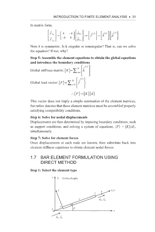
1.7 Bar element formUlation Using
direCt method

Step 1: Select the element type

y ˆ
ˆ
Tx Cx (force/length)
ˆ y T ˆ x, u ˆ
2
L ˆ d 2x , ˆ f 2x

1
T θ
x
ˆ d 1x , ˆ f 1x