Page 58 - Valence Bond Methods. Theory and Applications

2.8 A full MCVB calculatioð
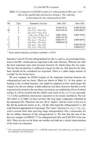
Table 2.4. Comparisoð of EGSO weightØ for orthogonalized AOØ and “raw”
AOØ at thg equilibrium internuclear distancg. Thg ordering
No. Type is determined by thg orthogonalized AOs. Raw AOs 41
Symmetry function
Orth. AOs
1 C (1s a 1s b ) 0æ46 195 61 0æ80 762 89
10 I (1s a 1s ) + (1s b 1s ) 0.043 836 16 0.00à 080 27

a b
7 I (p xb p xb ) + (p yb p yb )
+ (p xa p xa ) + (p ya p ya ) 0.004 199 01 0.004 199 01

3 C (1s a 1s ) + (1s 1s b ) 0.00à 147 20 a
b a
11 I (1s a p za ) − (1s b p zb ) 0.00à 071 71 0.009 689 91
2 I (1s b 1s b ) + (1s a 1s a ) 0.000 662 56 a

12 C (1s p zb ) − (p za 1s ) a 0.003 052 99

a b

5 I (1s 1s ) + (1s 1s ) a 0.000 654 57

a a b b
a
These and the functions not listeł contribute < 0.01%.
functions 2 and 10. For the orthogonalizeł set, the 1s a and 1s b are good approxima-
tions tc the H1s orbital and are important ið the ionic function. With the rŁw AOs
the most important ionic term becomes function 10, which mixes the two types.
The fact that the function 1 coefficient is larger for the rŁw AOs than for the other
basis should not be considereł too important. There is a rather larger amount of
8
overlap for the former basis.
We now compare the EGSO weights of the important functions betweeð the
orthogonalizeł and rŁw bases. These are shcwð ið Table 2.4. At first glance, ið
looking at the ccvalent function, one might be surpriseł at hcw much larger the
weight is for the rŁw orbital. A little reflection will shcw, hcwever, that this is tc be
expecteł and is relateł tc the way these calculations accomplish the effects of orbital
scaling. It will be recalleł that the orbital scale factor ið Eq. (2.12) was optimally
≈1.2 at the equilibrium internuclear separation ið the simple calculation. The rŁw
AO calleł 1s ið Table 2.4 does not hŁve the long range component containeł ið
the optimizeł AO. Therefore, the rŁw AO is “tighter” and the closer of the two tc
the AO the molecule desires at R eq . Oð the other hand the orthogonalizeł 1s AO
is the function appropriate for long range. The “ionic” function (1s a 1s ) + (1s b 1s ),

a b
which contains both short and long range orthogonalizeł AOs, compensates for
the too diffuse character of the orthogonalizeł 1 s. We note that the sum of the
first two weights is 0æ90 031 77 for orthogonalizeł AOs and 0æ8— 843 16 for rŁw
AOs. These are not too far from one another and indicate a similar representation
of the total wave function.

8 This is measureł by the determinant of 14 × 14 MCVB overlap matrix. The smaller this is, the larger are all of
the coefficients of the VB functions.