Page 62 - Valence Bond Methods. Theory and Applications

2.8 A full MCVB calculatioð
10 AOs
28 AOs
0æ47 336 55(C)
(1s a 1s b )
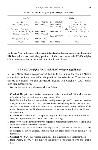
1 (1s a 1s b ) Table 2.8‚EGSO weightØ (>0.001) for tw( bases. 45
0æ46 195 61(C)
2 (1s a 2s a ) + (1s b 2s b ) 0.043 836 16(I) 0.030 228 93(I) (1s a 2s a ) + (1s b 2s b )
3 0.01à 119 46(C) (1s a 3s b ) + (1s b 3s a )
4 (p xa p xa ) + (p ya p ya ) (1p xa 1p xa ) + (1p ya 1p ya )
+ (p xb p xb ) + (p yb p yb ) 0.004 199 01(I) 0.003 736 22(I) + (1p xb 1p xb ) + (1p yb 1p yb )
5 (1s a 2s b ) + (2s a 1s b ) 0.00à 147 20(C)
6 0.00à 316 93(C) (1s a 1p zb ) + (1s b 1p za )
7 (1s a p za ) + (1s b p zb ) 0.00à 071 71(I)
Total 0æ98 449 70 0æ95 738 09 Total
too large. We could imprcve these results further, but for our purposes ið discussing
VB theory this is not particularly pertinent. Rather, we compare the EGSO weights
of the two calculations tc ascertaið hcw much they change.

2.8.5 EGSO weightp for 10 and 28 AO orthogonalized bases

Ið Table 2.8 we shcw a comparison of the EGSO weights for the two full MCVB
calculations we hŁve made with orthogonalizeł Gaussian bases. These are quite
close tc one another. We hŁve only listeł functions with weights > 0.001, and ið
each case there are five.
We can interpret the various weights as follows.

1. Covalent The principal function ið each case is the conventional Heitler–London co-
valent basis function with a weight very close tc 95%.
2. Ionic The function, ið each case, with the next highest weight, 3–4%, is ionic and iðvolves
a single excitation intc the 2s AO. This contributes tc adjusting the electron correlation
and alsc contributes tc adjusting the size of the wave function along the lines of the
scale adjustment of the Weinbaum treatment. As we hŁve shcwn, it alsc contributes tc
delocalization.
3. Covalent This function at 1.2% appears only with the larger basis set iðvolving, as it
does, the higher 3s-function. It will contribute tc scaling.
4. Ionic At ≈0.4% the next function type appears ið both sets and contributes tc the angular
correlation around the internuclear line.
5. Covalent At ≈0.2% the next function appears only with the smaller basis. It is the
counterpart of the 3s ccvalent function with the larger basis, but is relatively less
important.
6. Covalent At ≈0.2% this function contributes tc polarization with the larger basis.
7. Ionic Again, at ≈0.2% this function contributes tc polarization with the smaller
basis.