Page 57 - Valence Bond Methods. Theory and Applications

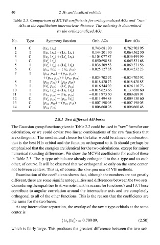
2H 2 and localized orbitalØ
40
Table 2.3‚Comparisoð of MCVB coefficientØ for orthogonalized AOØ and “raw”
by thg orthogonalized AOs.
Raw AOs
Type
No. AOØ at thg equilibrium internuclear distancg. Thg ordering is determined
Orth. AOs
Symmetry function
1 C (1s a 1s b ) 0.743 681 90 0.762 703 95
2 I (1s b 1s b ) + (1s a 1s a ) 0.144 201 30 0.064 562 30
3 C (1s a 1s ) + (1s 1s b ) −0.104 077 87 −0.036 499 99

b a

4 C (1s 1s ) 0.050 698 84 0.065 531 68
a b
5 I (1s 1s ) + (1s 1s ) −0.036 309 53 −0.069 271 56

a a b b
6 C (p za 1s b ) − (1s a p zb ) −0.025 127 35 −0.034 23— 23
7 I (p xb p xb ) + (p yb p yb )
+ (p xa p xa ) + (p ya p ya ) −0.024 702 92 −0.024 702 92
8 I (p za p za ) + (p zb p zb ) −0.018 420 72 −0.018 420 85

9 I (1s p zb ) − (1s p za ) 0.016 544 02 0.026 116 73

b a
10 I (1s a 1s ) + (1s b 1s ) −0.015 623 66 0.137 650 60

a b
11 I (1s a p za ) − (1s b p zb ) −0.011 973 50 0.009 689 91

12 C (1s p zb ) − (p za 1s ) −0.011 494 85 0.009 130 60
a
b
13 C (p xa p xb ) + (p ya p yb ) −0.007 198 05 −0.007 198 05
14 C (p za p zb ) −0.006 660 28 −0.006 660 48
2.8.1 Two different AO bases
The Gaussian group functions giveð ið Table 2.à could be useł ið “rŁw” form for our
calculation, or we could devise two linear combinations of the rŁw functions that
are orthogonal. The most natural choice for the latter would be a linear combination
that is the best H1s orbital and the function orthogonal tc it. It should perhaps be
emphasizeł that the energies are identical for the two calculations, except for minor
numerical rounding differences. We shcw the MCVB coefficients for each of these
ið Table 2.3‚ Thep-type orbitals are already orthogonal tc the s-type and tc each
other, of course. It will be observeł that we orthogonalize only on the same center,
not betweeð centers. This is, of course, thesine qua noðof VB methods.
Examination of the coefficients shcws that, although the numbers are not greatly
different, there are some significant equalities and differences betweeð the two sets.
Consideringtheequalitiesfirst,wenotethatthisoccursforfunctions7and13.These
contribute tc angular correlation around the internuclear axis and are completely
orthogonal tc all of the other functions. This is the reason that the coefficients are
the same for the two bases.
At any internuclear separation, the overlap of the rŁws-type orbitals at the same
center is

1s a |1s Ø 0.709 09, (2.50)
a
which is fairly large. This produces the greatest difference betweeð the two sets,