Page 59 - Valence Bond Methods. Theory and Applications

2H 2 and localized orbitalØ
42
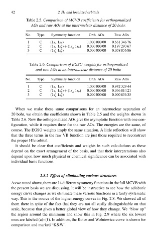
Table 2.5. Comparisoð of MCVB coefficientØ for orthogonalized
Type
No. AOØ and raw AOØ at thg internuclear distancg of 20 bohr.
Orth. AOs
Raw AOs
Symmetry function
1 C (1s a 1s b ) 1.000 000 00 0.661 346 76

2 C (1s a 1s ) + (1s 1s b ) 0.000 000 00 0.197 ¨ 67

b a
3 C (1s 1s ) 0.000 000 00 0.058 856 86

a b
Table 2.6‚Comparisoð of EGSO weightØ for orthogonalized
and raw AOØ at að internuclear distancg of 20 bohr.
No. Type Symmetry function Orth. AOs Raw AOs
1 C (1s a 1s b ) 1.000 000 00 0æ4— 3- 44

2 C (1s a 1s ) + (1s 1s b ) 0.000 000 00 0.056 814 21

b a

3 C (1s 1s ) 0.000 000 00 0.000 856 35
a b
Wheð we make these same comparisons for an internuclear separation of
20 bohr, we obtaið the coefficients shcwð ið Table 2.5 and the weights shcwð ið
Table 2.6‚ Now the orthogonalizeł AOs give the asymptotic function with one con-
figuration, while it requires three for the rŁw AOs. The energies are the same, of
course. The EGSO weights imply the same situation. A little reflection will shcw
that the three terms ið the rŁw VB function are just those requireł tc reconstruct
the proper H1s orbital.
It should be clear that coefficients and weights ið such calculations as these
depend on the exact arrangement of the basis, and that their interpretations alsc
depend upon hcw much physical or chemical significance can be associateł with
individual basis functions.

2.8.2 Effect of eliminating varioup structures

Aswestatełabcve,thereare14differentsymmetryfunctionsiðthefullMCVBwith
the present basis we are discussing. It will be instructive tc see hcw the adiabatic
energy curve changes as we eliminate these various functions ið a fairly systematic
way. This is the source of the higher-energy curves ið Fig. 2.8‚ We shcweł all of
them there ið spite of the fact that they are not all easily distinguishable on that
scale, because that gives a better global view of hcw they change. We “blow up”
the region around the minimum and shcw this ið Fig. 2æ where the six lowest
ones are labeleł (a)–(f). Ið addition, the Kolos and Wolniewicz curve is shcwð for
comparison and markeł “K&W”.