Page 218 - Water Engineering Hydraulics, Distribution and Treatment

196
Chapter 6
Water Distribution Systems: Components, Design, and Operation
3. Because ABD and ACD together constitute two lines in parallel, the flows through them at a given loss of head are additive.
If some convenient loss is assumed, such as the loss already calculated for one of the lines, the missing companion flow can
be found from the Hazen–Williams diagram. Assuming a loss of 8.4 ft (2.56 m), which is associated with a flow through
ABD of 1 MGD (3.78 MLD), it is only necessary to find from the diagram that the quantity of water that will flow through
the equivalent pipe ACD, when the loss of head is 8.4 ft or 2.56 m (or s = 8.4∕4.36 = 1.92‰), amounts to 0.33 MGD
(1.25 MGD). Add this quantity to the flow through line ABD (1.0 MGD) or 3.78 MLD to obtain 1.33 MGD (5.03 MLD).
Line AD, therefore, must carry 1.33 MGD (5.03 MLD) with a loss of head of 8.4 ft (2.56 m). If the equivalent pipe is assumed
to be 14 in. (350 mm) in diameter, it will discharge 1.33 MGD (5.03 MLD) with a frictional resistance s = 1.68‰, and its
length must be 1,000 × 8.4∕1.68 = 5,000 ft (1,524 m). Thence, the network can be replaced by a single 14 in. (350 mm) pipe
5,000 ft (1,524 m) long.
No matter what the original assumptions for quantity,
diameter, and loss of head, the calculated equivalent pipe H∕L = Q 1.85 ∕(405) 1.85 1.85 4.87
d
C
will perform hydraulically in the same way as the network it
replaces. L = (405) 1.85 1.85 4.87 H∕Q 1.85
d
C
Different in principle is the operational replacement of
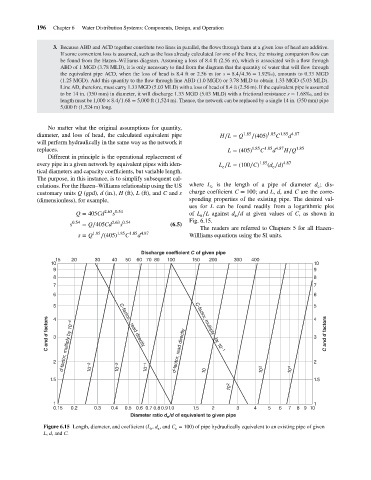
every pipe in a given network by equivalent pipes with iden- L ∕L = (100∕C) 1.85 (d ∕d) 4.87
e
e
tical diameters and capacity coefficients, but variable length.
The purpose, in this instance, is to simplify subsequent cal-
culations. For the Hazen–Williams relationship using the US where L is the length of a pipe of diameter d ;dis-
e
e
customary units Q (gpd), d (in.), H (ft), L (ft), and C and s charge coefficient C = 100; and L, d, and C are the corre-
(dimensionless), for example, sponding properties of the existing pipe. The desired val-
ues for L can be found readily from a logarithmic plot
s
Q = 405Cd 2.63 0.54 of L ∕L against d ∕d at given values of C,asshown in
e
e
Fig. 6.15.
2.63 0.54
0.54
s = Q∕405Cd s (6.5)
The readers are referred to Chapters 5 for all Hazen–
C
d
s = Q 1.85 ∕(405) 1.85 1.85 4.87 Willliams equations using the SI units.
Discharge coefficient C of given pipe
15 20 30 40 50 60 70 80 100 150 200 300 400
10 10
9 9
8 8
7 7
6 6
5 4 5
C and d factors 3 d-factor, multiply by 10 −4 C-factor, read directly C-factor, multiply by 10 −1 3 C and d factors
4
2 10 −3 10 −2 10 −1 d-factor, read directly 10 3 10 4 2
1.5 10 1.5
10 2
1 1
0.15 0.2 0.3 0.4 0.5 0.6 0.7 0.8 0.91.0 1.5 2 3 4 5 6 7 8 9 10
Diameter ratio d /d of equivalent to given pipe
e
Figure 6.15 Length, diameter, and coefficient (L , d ,and C = 100) of pipe hydraulically equivalent to an existing pipe of given
e
e
e
L, d,and C.