Page 213 - Water Engineering Hydraulics, Distribution and Treatment

191
6.6 Office Studies of Pipe Networks
The corrections q and h are only approximate. After they
the junctions being zero. If the assumed water table elevation
have been applied once to the assumed flows, the network
at a junction, such as the takeoff junction in Fig. 6.8b, is in
is more nearly in balance than it was at the beginning,
error by a height h, different small errors q are created in the
individual flows Q leading to and leaving from the junction.
but the process of correction must be repeated until the
n
n
For any one pipe, therefore, H + h = k(Q + q ) = kQ + h,
balancing operations are perfected. The work involved is
where H is the loss of head associated with the flow Q. More-
straightforward, but it is greatly facilitated by a satisfactory
scheme of bookkeeping such as that outlined for the method
over, as before,
of balancing heads in Example 6.3 for the network sketched
n−1
= nq(H∕Q) and
h = nkqQ
in Fig. 6.12.
q = (h∕n)(Q∕H)
Although the network in Example 6.3 is simple, it cannot
be solved conveniently by algebraic methods, because it con-
Because Σ(Q + q) = 0 at each junction,
tains two interfering hydraulic constituents: (a) a crossover
ΣQ =−Σq and
(pipe 4) involved in more than one circuit and (b) a series
Σq = (h∕n) Σ (Q∕H) ,or
of takeoffs representing water used along the pipelines, fire
ΣQ =− (h∕n) Σ (Q∕H) , therefore, flows through hydrants, or supplies through to neighboring
circuits.
nΣQ
h =− (6.4)
Σ (Q∕H)
EXAMPLE 6.3 ANALYSIS OF A WATER NETWORK USING THE RELAXATION METHOD OF BALANCING
HEADS
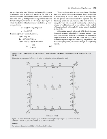
Balance the network shown in Figure 6.12 using the relaxation method of balancing heads
Take-off
Q 0 Q 1 Q 2 Q 3
Inflow
2.0
1.00 1.21 1.24 1.25 0.6
A 1. 2000´−12˝ B
Q 3 0.75 Q 3 0.65 1000´−8˝
Q 2 0.76 1000´−8˝ I Q 2 0.64
Q 1 0.79 Q 1 0.61
3. 2.
Q 0 1.00 Q 0 Q 1 Q 2 Q 3 Q 0 0.40
C
0.50 0.36 0.36 0.36 Take-off
4. 2000´−8˝ 0.6
Q 3 0.39 1000´−6˝ Q 3 0.41 1000´−6˝
Q 2 0.40 II Q 2 0.40
Q 1 0.43 Q 1 0.37
6. 5.
Q 0 0.50 Q 0 0.30
Q 0
Q 3
Q 1
Q 2
D 0.30 0.23 0.20 0.19 E
Take-off 0.2 7. 2000´−6˝ 0.6
Take-off
All flows are in MGD
Figure 6.12 Plan of network analyzed by the method of balancing heads (Example 6.3). Conversion factors:
′′
′
1MGD = 3.785 MLD; 1 = 1ft = 0.3048 m; 1 = 1in. = 25.4 mm.
Solution:
The schedule of calculations (Table 6.4) includes the following: