Page 212 - Water Engineering Hydraulics, Distribution and Treatment

190
Water Distribution Systems: Components, Design, and Operation
Chapter 6
(d) Pipes added: two 10 in. (250 mm) at 0.6MGD = 1.2 MGD (4.5 MLD).
Pipes removed: one 6 in. at 0.2 MGD (one 150 mm at 0.76 MLD).
Net added capacity: 1.2 − 0.2 = 1.0 MGD (3.8 MLD).
Reinforced capacity = 6.5 + 1.0 = 7.5MGD or (24.6 + 3.8 = 28.4 MLD).
(e) The reinforced system equivalent pipe at 7.5 MGD (28.4 MLD) and a hydraulic gradient of 2‰ is 26.0 in. (650 mm)
This will carry 7.6 MGD (28.8 MLD) with a loss of head of 2.1‰.
6.6.2 Relaxation (Hardy Cross)
Two procedures may be involved, depending on whether
A method of relaxation,or controlled trial and error,was
introduced by Hardy Cross, whose procedures are followed (a) the quantities of water entering and leaving the network or
(b) the piezometric levels, pressures,or water table elevations
here with only a few modifications. In applying a method
at inlets and outlets are known.
of this kind, calculations become speedier if pipe–flow
In balancing heads by correcting assumed flows, neces-
relationships are expressed by an exponential formula with
sary formulations are made algebraically consistent by arbi-
unvarying capacity coefficient, and notation becomes simpler
trarily assigning positive signs to clockwise flows and asso-
if the exponential formula is written:
ciated head losses, and negative signs to counterclockwise
H = kQ n (6.1) flows and associated head losses. For the simple network
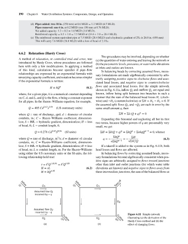
shown in Fig. 6.11a, inflow Q and outflow Q are equal and
i o
where, for a given pipe, k is a numerical constant depending known, inflow being split between two branches in such a
on C, d, and L, and Q is the flow, n being a constant exponent manner that the sum of the balanced head losses H (clock-
1
for all pipes. In the Hazen–Williams equation, for example, wise) and −H (counterclockwise) or ΣH = H − H = 0. If
2
1
2
the assumed split flows Q and −Q are each in error by the
2
1
Q = 405 Cd 2.63 0.54 (US customary units) same small amount q, then
s
n
where Q = rate of discharge, gpd; d = diameter of circular ΣH =Σk (Q + q) = 0
conduits, in.; C = Hazen–Williams coefficient, dimension- Expanding this binomial and neglecting all but its first
less; S = H/L = hydraulic gradient, dimensionless; H = loss two terms, because higher powers of q are presumably very
of head, ft; L = conduit length, ft. small, we get
n
n
S
Q = 0.278 Cd 2.63 0.54 (SI units) ΣH =Σk(Q + q) =ΣkQ +ΣnkqQ n−1 = 0, whence
ΣkQ n ΣH
3
where Q = rate of discharge, m /s; d = diameter of circular q =− n−1 =− (6.3)
conduits, m; C = Hazen–Williams coefficient, dimension- nΣkQ nΣH∕Q
less; S = H/L = hydraulic gradient, dimensionless; H = loss If a takeoff is added to the system as in Fig. 6.11b, both
of head, m; L = conduit length, m. For the Hazen–Williams head losses and flows are affected.
using either the US customary units or the SI units, the fol- In balancing flows by correcting assumed heads, neces-
lowing relationship hold true: sary formulations become algebraically consistent when pos-
itive signs are arbitrarily assigned to flows toward junctions
′
′
s = k Q 1∕0.54 = k Q 1.85 other than inlet and outlet junctions (for which water table
H = sL (6.2) elevations are known) and negative signs to flows away from
H = kQ 1.85 these intermediate junctions, the sum of the balanced flows at
Take-off
Q i Q 1 Q i Q 1 T
Inflow
Inflow
Assumed flow Q i
incorrect by + q
Q 3
Assumed flow Q 2
incorrect by – q
Figure 6.11 Simple network
Q 2 Q o Q 2 Q Outflow illustrating (a) the derivation of the
o
Outflow
Hardy Cross method and (b) the
(a) (b) effect of changing flows.